Stochastic Solver¶

When a quantum system is subjected to continuous measurement, through homodyne detection for example, it is possible to simulate the conditional quantum state using stochastic Schrodinger and master equations. The solution of these stochastic equations are quantum trajectories, which represent the conditioned evolution of the system given a specific measurement record.

In general, the stochastic evolution of a quantum state is calculated in QuTiP by solving the general equation

(1)¶\[d \rho (t) = d_1 \rho dt + \sum_n d_{2,n} \rho dW_n,\]

where \(dW_n\) is a Wiener increment, which has the expectation values \(E[dW] = 0\) and \(E[dW^2] = dt\). Stochastic evolution is implemented with the qutip.stochastic.general_stochastic function.

Stochastic Schrodinger Equation¶

The stochastic Schrodinger equation is given by (see section 4.4, [Wis09])

(2)¶\[d \psi(t) = - i H \psi(t) dt - \sum_n \left( \frac{S_n^\dagger S_n}{2} -\frac{e_n}{2} S_n + \frac{e_n^2}{8} \right) \psi(t) dt + \sum_n \left( S_n - \frac{e_n}{2} \right) \psi(t) dW_n,\]

where \(H\) is the Hamiltonian, \(S_n\) are the stochastic collapse operators, and \(e_n\) is

(3)¶\[e_n = \left<\psi(t)|S_n + S_n^\dagger|\psi(t)\right>\]

In QuTiP, this equation can be solved using the function qutip.stochastic.ssesolve, which is implemented by defining \(d_1\) and \(d_{2,n}\) from Equation (1) as

(4)¶\[d_1 = -iH - \frac{1}{2} \sum_n \left(S_n^\dagger S_n - e_n S_n + \frac{e_i^2}{4} \right),\]

and

(5)¶\[d_{2, n} = S_n - \frac{e_n}{2}.\]

The solver qutip.stochastic.ssesolve will construct the operators \(d_1\) and \(d_{2,n}\) once the user passes the Hamiltonian (H) and the stochastic operator list (sc_ops). As with the qutip.mcsolve, the number of trajectories and the seed for the noise realisation can be fixed using the arguments: ntraj and noise, respectively. If the user also requires the measurement output, the argument store_measurement=True should be included.

Additionally, homodyne and heterodyne detections can be easily simulated by passing the arguments method='homodyne' or method='heterodyne' to qutip.stochastic.ssesolve.

Examples of how to solve the stochastic Schrodinger equation using QuTiP can be found in this development notebook.

Stochastic Master Equation¶

When the initial state of the system is a density matrix \(\rho\), the stochastic master equation solver qutip.stochastic.smesolve must be used. The stochastic master equation is given by (see section 4.4, [Wis09])

(6)¶\[ d \rho (t) = -i[H, \rho(t)] dt + D[A]\rho(t) dt + \mathcal{H}[A]\rho dW(t)\]

where

(7)¶\[D[A] \rho = \frac{1}{2} \left[2 A \rho A^\dagger - \rho A^\dagger A - A^\dagger A \rho \right],\]

and

(8)¶\[\mathcal{H}[A]\rho = A\rho(t) + \rho(t) A^\dagger - \tr[A\rho(t) + \rho(t) A^\dagger].\]

In QuTiP, solutions for the stochastic master equation are obtained using the solver qutip.stochastic.smesolve. The implementation takes into account 2 types of collapse operators. \(C_i\) (c_ops) represent the dissipation in the environment, while \(S_n\) (sc_ops) are monitored operators. The deterministic part of the evolution, described by the \(d_1\) in Equation (1), takes into account all operators \(C_i\) and \(S_n\):

(9)¶\[d_1 = - i[H(t),\rho(t)] + \sum_i D[C_i]\rho + \sum_n D[S_n]\rho,\]

The stochastic part, \(d_{2,n}\), is given solely by the operators \(S_n\)

(10)¶\[d_{2,n} = S_n \rho(t) + \rho(t) S_n^\dagger - \tr \left(S_n \rho (t) + \rho(t) S_n^\dagger \right)\rho(t).\]

As in the stochastic Schrodinger equation, the detection method can be specified using the method argument.

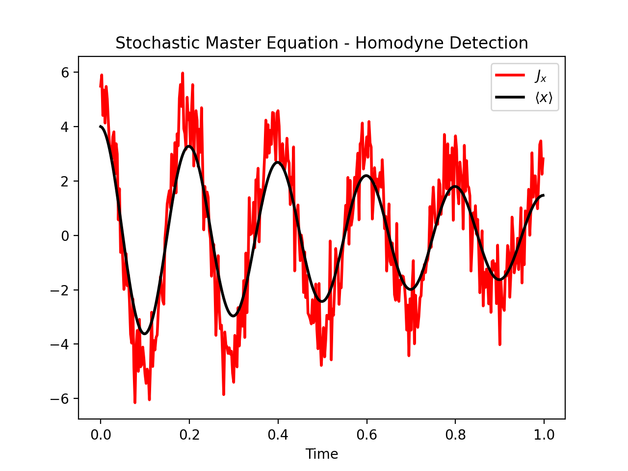
Example¶

Below, we solve the dynamics for an optical cavity at 0K whose output is monitored using homodyne detection. The cavity decay rate is given by \(\kappa\) and the \(\Delta\) is the cavity detuning with respect to the driving field. The measurement operators can be passed using the option m_ops. The homodyne current \(J_x\) is calculated using

(11)¶\[J_x = \langle x \rangle + dW,\]

where \(x\) is the operator passed using m_ops. The results are available in result.measurements.

import numpy as np
import matplotlib.pyplot as plt
import qutip as qt

# parameters
DIM = 20             # Hilbert space dimension
DELTA = 5*2*np.pi    # cavity detuning
KAPPA = 2            # cavity decay rate
INTENSITY = 4        # intensity of initial state
NUMBER_OF_TRAJECTORIES = 500

# operators
a = qt.destroy(DIM)
x = a + a.dag()
H = DELTA*a.dag()* a

rho_0 = qt.coherent(DIM, np.sqrt(INTENSITY))
times = np.arange(0, 1, 0.0025)

stoc_solution = qt.smesolve(H, rho_0, times,
                            c_ops=[],
                            sc_ops=[np.sqrt(KAPPA) * a],
                            e_ops=[x],
                            ntraj=NUMBER_OF_TRAJECTORIES,
                            nsubsteps=2,
                            store_measurement=True,
                            dW_factors=[1],
                            method='homodyne')

fig, ax = plt.subplots()
ax.set_title('Stochastic Master Equation - Homodyne Detection')
ax.plot(times, np.array(stoc_solution.measurement).mean(axis=0)[:].real,
        'r', lw=2, label=r'$J_x$')
ax.plot(times, stoc_solution.expect[0], 'k', lw=2,
        label=r'$\langle x \rangle$')
ax.set_xlabel('Time')
ax.legend()

(png, hires.png, pdf)

For other examples on qutip.stochastic.smesolve, see the following notebook, as well as these notebooks available at QuTiP Tutorials page: heterodyne detection, inneficient detection, and feedback control.