Saving QuTiP Objects and Data Sets
With time-consuming calculations it is often necessary to store the results to files on disk, so it can be post-processed and archived. In QuTiP there are two facilities for storing data: Quantum objects can be stored to files and later read back as python pickles, and numerical data (vectors and matrices) can be exported as plain text files in for example CSV (comma-separated values), TSV (tab-separated values), etc. The former method is preferred when further calculations will be performed with the data, and the latter when the calculations are completed and data is to be imported into a post-processing tool (e.g. for generating figures).
Storing and loading QuTiP objects
To store and load arbitrary QuTiP related objects (qutip.Qobj, qutip.solver.Result, etc.) there are two functions: qutip.fileio.qsave and qutip.fileio.qload. The function qutip.fileio.qsave takes an arbitrary object as first parameter and an optional filename as second parameter (default filename is qutip_data.qu). The filename extension is always .qu. The function qutip.fileio.qload takes a mandatory filename as first argument and loads and returns the objects in the file.
To illustrate how these functions can be used, consider a simple calculation of the steadystate of the harmonic oscillator
>>> a = destroy(10); H = a.dag() * a
>>> c_ops = [np.sqrt(0.5) * a, np.sqrt(0.25) * a.dag()]
>>> rho_ss = steadystate(H, c_ops)
The steadystate density matrix rho_ss is an instance of qutip.Qobj. It can be stored to a file steadystate.qu using
>>> qsave(rho_ss, 'steadystate')
>>> !ls *.qu
density_matrix_vs_time.qu  steadystate.qu
and it can later be loaded again, and used in further calculations
>>> rho_ss_loaded = qload('steadystate')
Loaded Qobj object:
Quantum object: dims = [[10], [10]], shape = (10, 10), type = oper, isHerm = True
>>> a = destroy(10)
>>> np.testing.assert_almost_equal(expect(a.dag() * a, rho_ss_loaded), 0.9902248289345061)
The nice thing about the qutip.fileio.qsave and qutip.fileio.qload functions is that almost any object can be stored and load again later on. We can for example store a list of density matrices as returned by qutip.mesolve
>>> a = destroy(10); H = a.dag() * a ; c_ops = [np.sqrt(0.5) * a, np.sqrt(0.25) * a.dag()]
>>> psi0 = rand_ket(10)
>>> times = np.linspace(0, 10, 10)
>>> dm_list = mesolve(H, psi0, times, c_ops, [])
>>> qsave(dm_list, 'density_matrix_vs_time')
And it can then be loaded and used again, for example in an other program
>>> dm_list_loaded = qload('density_matrix_vs_time')
Loaded Result object:
Result object with mesolve data.
--------------------------------
states = True
num_collapse = 0
>>> a = destroy(10)
>>> expect(a.dag() * a, dm_list_loaded.states)
array([4.63317086, 3.59150315, 2.90590183, 2.41306641, 2.05120716,
   1.78312503, 1.58357995, 1.4346382 , 1.32327398, 1.23991233])
Storing and loading datasets
The qutip.fileio.qsave and qutip.fileio.qload are great, but the file format used is only understood by QuTiP (python) programs. When data must be exported to other programs the preferred method is to store the data in the commonly used plain-text file formats. With the QuTiP functions qutip.fileio.file_data_store and qutip.fileio.file_data_read we can store and load numpy arrays and matrices to files on disk using a deliminator-separated value format (for example comma-separated values CSV). Almost any program can handle this file format.
The qutip.fileio.file_data_store takes two mandatory and three optional arguments:
>>> file_data_store(filename, data, numtype="complex", numformat="decimal", sep=",")
where filename is the name of the file, data is the data to be written to the file (must be a numpy array), numtype (optional) is a flag indicating numerical type that can take values complex or real, numformat (optional) specifies the numerical format that can take the values exp for the format 1.0e1 and decimal for the format 10.0, and sep (optional) is an arbitrary single-character field separator (usually a tab, space, comma, semicolon, etc.).
A common use for the qutip.fileio.file_data_store function is to store the expectation values of a set of operators for a sequence of times, e.g., as returned by the qutip.mesolve function, which is what the following example does
>>> a = destroy(10); H = a.dag() * a ; c_ops = [np.sqrt(0.5) * a, np.sqrt(0.25) * a.dag()]
>>> psi0 = rand_ket(10)
>>> times = np.linspace(0, 100, 100)
>>> medata = mesolve(H, psi0, times, c_ops, [a.dag() * a, a + a.dag(), -1j * (a - a.dag())])
>>> np.shape(medata.expect)
(3, 100)
>>> times.shape
(100,)
>>> output_data = np.vstack((times, medata.expect))   # join time and expt data
>>> file_data_store('expect.dat', output_data.T) # Note the .T for transpose!
>>> with open("expect.dat", "r") as f:
...    print('\n'.join(f.readlines()[:10]))
# Generated by QuTiP: 100x4 complex matrix in decimal format [',' separated values].
0.0000000000+0.0000000000j,3.2109553666+0.0000000000j,0.3689771549+0.0000000000j,0.0185002867+0.0000000000j
1.0101010101+0.0000000000j,2.6754598872+0.0000000000j,0.1298251132+0.0000000000j,-0.3303672956+0.0000000000j
2.0202020202+0.0000000000j,2.2743186810+0.0000000000j,-0.2106241300+0.0000000000j,-0.2623894277+0.0000000000j
3.0303030303+0.0000000000j,1.9726633457+0.0000000000j,-0.3037311621+0.0000000000j,0.0397330921+0.0000000000j
4.0404040404+0.0000000000j,1.7435892209+0.0000000000j,-0.1126550232+0.0000000000j,0.2497182058+0.0000000000j
5.0505050505+0.0000000000j,1.5687324121+0.0000000000j,0.1351622725+0.0000000000j,0.2018398581+0.0000000000j
6.0606060606+0.0000000000j,1.4348632045+0.0000000000j,0.2143080535+0.0000000000j,-0.0067820038+0.0000000000j
7.0707070707+0.0000000000j,1.3321818015+0.0000000000j,0.0950352763+0.0000000000j,-0.1630920429+0.0000000000j
8.0808080808+0.0000000000j,1.2533244850+0.0000000000j,-0.0771210981+0.0000000000j,-0.1468923919+0.0000000000j
In this case we didn’t really need to store both the real and imaginary parts, so instead we could use the numtype="real" option
>>> file_data_store('expect.dat', output_data.T, numtype="real")
>>> with open("expect.dat", "r") as f:
...    print('\n'.join(f.readlines()[:5]))
# Generated by QuTiP: 100x4 real matrix in decimal format [',' separated values].
0.0000000000,3.2109553666,0.3689771549,0.0185002867
1.0101010101,2.6754598872,0.1298251132,-0.3303672956
2.0202020202,2.2743186810,-0.2106241300,-0.2623894277
3.0303030303,1.9726633457,-0.3037311621,0.0397330921
and if we prefer scientific notation we can request that using the numformat="exp" option
>>> file_data_store('expect.dat', output_data.T, numtype="real", numformat="exp")
Loading data previously stored using qutip.fileio.file_data_store (or some other software) is a even easier. Regardless of which deliminator was used, if data was stored as complex or real numbers, if it is in decimal or exponential form, the data can be loaded using the qutip.fileio.file_data_read, which only takes the filename as mandatory argument.
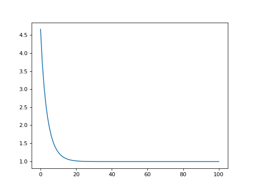
input_data = file_data_read('expect.dat')
plt.plot(input_data[:,0], input_data[:,1]);  # plot the data
(If a particularly obscure choice of deliminator was used it might be necessary to use the optional second argument, for example sep="_" if _ is the deliminator).