Krylov Solver¶

Introduction¶

The Krylov-subspace method is a standard method to approximate quantum dynamics. Let \(\left|\psi\right\rangle\) be a state in a \(D\)-dimensional complex Hilbert space that evolves under a time-independent Hamiltonian \(H\). Then, the \(N\)-dimensional Krylov subspace associated with that state and Hamiltonian is given by

(1)¶\[\mathcal{K}_{N}=\operatorname{span}\left\{|\psi\rangle, H|\psi\rangle, \ldots, H^{N-1}|\psi\rangle\right\},\]

where the dimension \(N<D\) is a parameter of choice. To construct an orthonormal basis \(B_N\) for \(\mathcal{K}_{N}\), the simplest algorithm is the well-known Lanczos algorithm, which provides a sort of Gram-Schmidt procedure that harnesses the fact that orthonormalization needs to be imposed only for the last two vectors in the basis. Written in this basis the time-evolved state can be approximated as

(2)¶\[|\psi(t)\rangle=e^{-iHt}|\psi\rangle\approx\mathbb{P}_{N}e^{-iHt}\mathbb{P}_{N}|\psi\rangle=\mathbb{V}_{N}^{\dagger}e^{-iT_{N}t}\mathbb{V}_{N}|\psi\rangle\equiv\left|\psi_{N}(t)\right\rangle,\]

where \(T_{N}=\mathbb{V}_{N} H \mathbb{V}_{N}^{\dagger}\) is the Hamiltonian reduced to the Krylov subspace (which takes a tridiagonal matrix form), and \(\mathbb{V}_{N}^{\dagger}\) is the matrix containing the vectors of the Krylov basis as columns.

With the above approximation, the time-evolution is calculated only with a smaller square matrix of the desired size. Therefore, the Krylov method provides huge speed-ups in computation of short-time evolutions when the dimension of the Hamiltonian is very large, a point at which exact calculations on the complete subspace are practically impossible.

One of the biggest problems with this type of method is the control of the error. After a short time, the error starts to grow exponentially. However, this can be easily corrected by restarting the subspace when the error reaches a certain threshold. Therefore, a series of \(M\) Krylov-subspace time evolutions provides accurate solutions for the complete time evolution. Within this scheme, the magic of Krylov resides not only in its ability to capture complex time evolutions from very large Hilbert spaces with very small dimenions \(M\), but also in the computing speed-up it presents.

For exceptional cases, the Lanczos algorithm might arrive at the exact evolution of the initial state at a dimension \(M_{hb}<M\). This is called a happy breakdown. For example, if a Hamiltonian has a symmetry subspace \(D_{\text{sim}}<M\), then the algorithm will optimize using the value math:M_{hb}<M:, at which the evolution is not only exact but also cheap.

Krylov Solver in QuTiP¶

In QuTiP, Krylov-subspace evolution is implemented as the function qutip.krylovsolve. Arguments are nearly the same as qutip.mesolve function for master-equation evolution, except that the initial state must be a ket vector, as opposed to a density matrix, and the additional parameter krylov_dim that defines the maximum allowed Krylov-subspace dimension. The maximum number of allowed Lanczos partitions can also be determined using the qutip.solver.options.nsteps parameter, which defaults to ‘10000’.

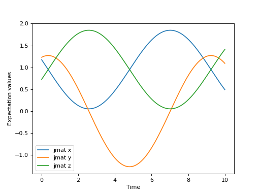
Let’s solve a simple example using the algorithm in QuTiP to get familiar with the method.

>>> from qutip import jmat, rand_ket, krylovsolve
>>> import numpy as np
>>> import matplotlib.pyplot as plt
>>> dim = 100
>>> e_ops = [jmat((dim - 1) / 2.0, "x"), jmat((dim - 1) / 2.0, "y"), jmat((dim - 1) / 2.0, "z")]
>>> H = .5*jmat((dim - 1) / 2.0, "z") + .5*jmat((dim - 1) / 2.0, "x")
>>> psi0 = rand_ket(dim)
>>> tlist = np.linspace(0.0, 10.0, 200)
>>> results = krylovsolve(H, psi0, tlist, krylov_dim=20, e_ops=e_ops)
>>> plt.figure()
>>> for expect in results.expect:
>>>    plt.plot(tlist, expect)
>>> plt.legend(('jmat x', 'jmat y', 'jmat z'))
>>> plt.xlabel('Time')
>>> plt.ylabel('Expectation values')
>>> plt.show()

Sparse and Dense Hamiltonians¶

If the Hamiltonian of interest is known to be sparse, qutip.krylovsolve also comes equipped with the possibility to store its internal data in a sparse optimized format using scipy. This allows for significant speed-ups, let’s showcase it:

>>> from qutip import krylovsolve, rand_herm, rand_ket
>>> import numpy as np
>>> from time import time
>>> def time_krylov(psi0, H, tlist, sparse):
>>>     start = time()
>>>     krylovsolve(H, psi0, tlist, krylov_dim=30, sparse=sparse)
>>>     end = time()
>>>     return end - start
>>> dim = 2000
>>> tlist = np.linspace(0, 1, 10)
>>> psi0 = rand_ket(dim, seed=0)
>>> H_sparse = rand_herm(dim, density=0.1, seed=0)
>>> H_dense = rand_herm(dim, density=0.9, seed=0)
>>> # first index for type of H and second index for sparse = True or False (dense)
>>> t_ss = time_krylov(psi0, H_sparse, tlist, sparse=True)
>>> t_sd = time_krylov(psi0, H_sparse, tlist, sparse=False)
>>> t_ds = time_krylov(psi0, H_dense, tlist, sparse=True)
>>> t_dd = time_krylov(psi0, H_dense, tlist, sparse=False)
>>> print(f"Average time of solution for a sparse H is {round((t_sd)/t_ss, 2)} faster for sparse=True in comparison to sparse=False")
>>> print(f"Average time of solution for a dense H is {round((t_dd)/t_ds, 2)} slower for sparse=True in comparison to sparse=False")
Average time of solution for a sparse H is 2.46 faster for sparse=True in comparison to sparse=False
Average time of solution for a dense H is 0.45 slower for sparse=True in comparison to sparse=False