Two-time correlation functions
With the QuTiP time-evolution functions (for example qutip.mesolve and qutip.mcsolve), a state vector or density matrix can be evolved from an initial state at \(t_0\) to an arbitrary time \(t\), \(\rho(t)=V(t, t_0)\left\{\rho(t_0)\right\}\), where \(V(t, t_0)\) is the propagator defined by the equation of motion. The resulting density matrix can then be used to evaluate the expectation values of arbitrary combinations of same-time operators.
To calculate two-time correlation functions on the form \(\left<A(t+\tau)B(t)\right>\), we can use the quantum regression theorem (see, e.g., [Gar03]) to write
We therefore first calculate \(\rho(t)=V(t, 0)\left\{\rho(0)\right\}\) using one of the QuTiP evolution solvers with \(\rho(0)\) as initial state, and then again use the same solver to calculate \(V(t+\tau, t)\left\{B\rho(t)\right\}\) using \(B\rho(t)\) as initial state.
Note that if the initial state is the steady state, then \(\rho(t)=V(t, 0)\left\{\rho_{\rm ss}\right\}=\rho_{\rm ss}\) and
which is independent of \(t\), so that we only have one time coordinate \(\tau\).
QuTiP provides a family of functions that assists in the process of calculating two-time correlation functions. The available functions and their usage is shown in the table below. Each of these functions can use one of the following evolution solvers: Master-equation, Exponential series and the Monte-Carlo. The choice of solver is defined by the optional argument solver.
QuTiP function |
Correlation function |
|---|---|
|
\(\left<A(t+\tau)B(t)\right>\) or \(\left<A(t)B(t+\tau)\right>\). |
|
\(\left<A(\tau)B(0)\right>\) or \(\left<A(0)B(\tau)\right>\). |
\(\left<A(0)B(\tau)C(\tau)D(0)\right>\). |
|
\(\left<A(t)B(t+\tau)C(t+\tau)D(t)\right>\). |
The most common use-case is to calculate correlation functions of the kind \(\left<A(\tau)B(0)\right>\), in which case we use the correlation function solvers that start from the steady state, e.g., the qutip.correlation.correlation_2op_1t function. These correlation function solvers return a vector or matrix (in general complex) with the correlations as a function of the delays times.
Steadystate correlation function
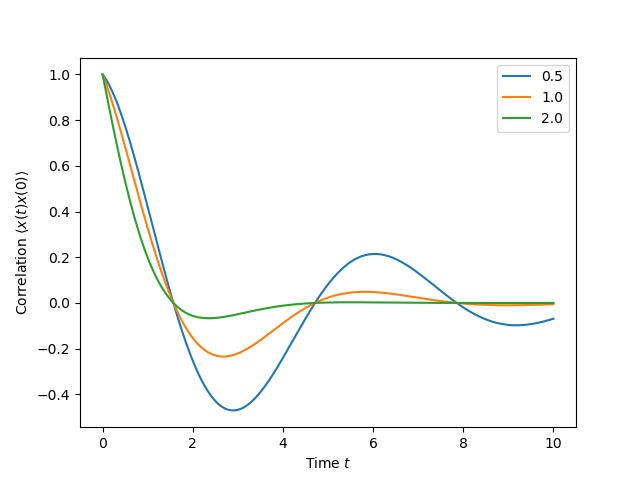
The following code demonstrates how to calculate the \(\left<x(t)x(0)\right>\) correlation for a leaky cavity with three different relaxation rates.
In [1]: times = np.linspace(0,10.0,200)

In [2]: a = destroy(10)

In [3]: x = a.dag() + a

In [4]: H = a.dag() * a

In [5]: corr1 = correlation_2op_1t(H, None, times, [np.sqrt(0.5) * a], x, x)

In [6]: corr2 = correlation_2op_1t(H, None, times, [np.sqrt(1.0) * a], x, x)

In [7]: corr3 = correlation_2op_1t(H, None, times, [np.sqrt(2.0) * a], x, x)

In [8]: figure()
Out[8]: <Figure size 640x480 with 0 Axes>

In [9]: plot(times, np.real(corr1), times, np.real(corr2), times, np.real(corr3))
Out[9]:
[<matplotlib.lines.Line2D at 0x1a26dd45f8>,
 <matplotlib.lines.Line2D at 0x1a26dd4668>,
 <matplotlib.lines.Line2D at 0x1a250d2c18>]

In [10]: legend(['0.5','1.0','2.0'])
Out[10]: <matplotlib.legend.Legend at 0x1a2551cef0>

In [11]: xlabel(r'Time $t$')
Out[11]: Text(0.5,0,'Time $t$')

In [12]: ylabel(r'Correlation $\left<x(t)x(0)\right>$')
Out[12]: Text(0,0.5,'Correlation $\\left<x(t)x(0)\\right>$')

In [13]: show()
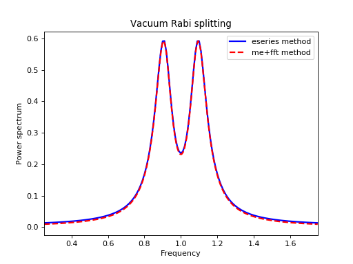
Emission spectrum
Given a correlation function \(\left<A(\tau)B(0)\right>\) we can define the corresponding power spectrum as
In QuTiP, we can calculate \(S(\omega)\) using either qutip.correlation.spectrum_ss, which first calculates the correlation function using the qutip.essolve.essolve solver and then performs the Fourier transform semi-analytically, or we can use the function qutip.correlation.spectrum_correlation_fft to numerically calculate the Fourier transform of a given correlation data using FFT.
The following example demonstrates how these two functions can be used to obtain the emission power spectrum.
import numpy as np
import pylab as plt
from qutip import *

N = 4                   # number of cavity fock states
wc = wa = 1.0 * 2 * np.pi  # cavity and atom frequency
g  = 0.1 * 2 * np.pi       # coupling strength
kappa = 0.75            # cavity dissipation rate
gamma = 0.25            # atom dissipation rate

# Jaynes-Cummings Hamiltonian
a  = tensor(destroy(N), qeye(2))
sm = tensor(qeye(N), destroy(2))
H = wc * a.dag() * a + wa * sm.dag() * sm + g * (a.dag() * sm + a * sm.dag())

# collapse operators
n_th = 0.25
c_ops = [np.sqrt(kappa * (1 + n_th)) * a, np.sqrt(kappa * n_th) * a.dag(), np.sqrt(gamma) * sm]

# calculate the correlation function using the mesolve solver, and then fft to
# obtain the spectrum. Here we need to make sure to evaluate the correlation
# function for a sufficient long time and sufficiently high sampling rate so
# that the discrete Fourier transform (FFT) captures all the features in the
# resulting spectrum.
tlist = np.linspace(0, 100, 5000)
corr = correlation_2op_1t(H, None, tlist, c_ops, a.dag(), a)
wlist1, spec1 = spectrum_correlation_fft(tlist, corr)


# calculate the power spectrum using spectrum, which internally uses essolve
# to solve for the dynamics (by default)
wlist2 = np.linspace(0.25, 1.75, 200) * 2 * np.pi
spec2 = spectrum(H, wlist2, c_ops, a.dag(), a)

# plot the spectra
fig, ax = plt.subplots(1, 1)
ax.plot(wlist1 / (2 * np.pi), spec1, 'b', lw=2, label='eseries method')
ax.plot(wlist2 / (2 * np.pi), spec2, 'r--', lw=2, label='me+fft method')
ax.legend()
ax.set_xlabel('Frequency')
ax.set_ylabel('Power spectrum')
ax.set_title('Vacuum Rabi splitting')
ax.set_xlim(wlist2[0]/(2*np.pi), wlist2[-1]/(2*np.pi))
plt.show()
(Source code, png, hires.png, pdf)

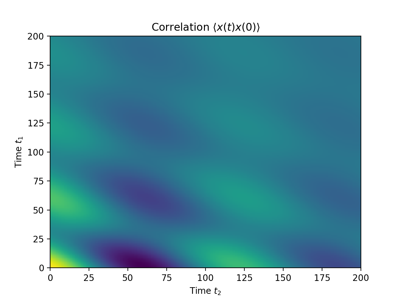
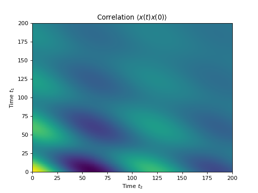
Non-steadystate correlation function
More generally, we can also calculate correlation functions of the kind \(\left<A(t_1+t_2)B(t_1)\right>\), i.e., the correlation function of a system that is not in its steadystate. In QuTiP, we can evoluate such correlation functions using the function qutip.correlation.correlation_2op_2t. The default behavior of this function is to return a matrix with the correlations as a function of the two time coordinates (\(t_1\) and \(t_2\)).
import numpy as np
import pylab as plt
from qutip import *

times = np.linspace(0, 10.0, 200)
a = destroy(10)
x = a.dag() + a
H = a.dag() * a
alpha = 2.5
rho0 = coherent_dm(10, alpha)
corr = correlation_2op_2t(H, rho0, times, times, [np.sqrt(0.25) * a], x, x)

plt.pcolor(np.real(corr))
plt.xlabel(r'Time $t_2$')
plt.ylabel(r'Time $t_1$')
plt.title(r'Correlation $\left<x(t)x(0)\right>$')
plt.show()
(Source code, png, hires.png, pdf)
However, in some cases we might be interested in the correlation functions on the form \(\left<A(t_1+t_2)B(t_1)\right>\), but only as a function of time coordinate \(t_2\). In this case we can also use the qutip.correlation.correlation_2op_2t function, if we pass the density matrix at time \(t_1\) as second argument, and None as third argument. The qutip.correlation.correlation_2op_2t function then returns a vector with the correlation values corresponding to the times in taulist (the fourth argument).
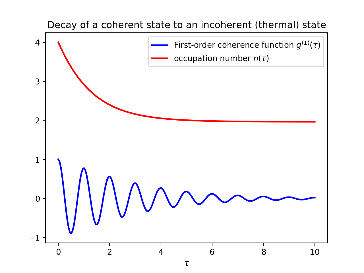
Example: first-order optical coherence function
This example demonstrates how to calculate a correlation function on the form \(\left<A(\tau)B(0)\right>\) for a non-steady initial state. Consider an oscillator that is interacting with a thermal environment. If the oscillator initially is in a coherent state, it will gradually decay to a thermal (incoherent) state. The amount of coherence can be quantified using the first-order optical coherence function \(g^{(1)}(\tau) = \frac{\left<a^\dagger(\tau)a(0)\right>}{\sqrt{\left<a^\dagger(\tau)a(\tau)\right>\left<a^\dagger(0)a(0)\right>}}\). For a coherent state \(|g^{(1)}(\tau)| = 1\), and for a completely incoherent (thermal) state \(g^{(1)}(\tau) = 0\). The following code calculates and plots \(g^{(1)}(\tau)\) as a function of \(\tau\).
import numpy as np
import pylab as plt
from qutip import *

N = 15
taus = np.linspace(0,10.0,200)
a = destroy(N)
H = 2 * np.pi * a.dag() * a

# collapse operator
G1 = 0.75
n_th = 2.00  # bath temperature in terms of excitation number
c_ops = [np.sqrt(G1 * (1 + n_th)) * a, np.sqrt(G1 * n_th) * a.dag()]

# start with a coherent state
rho0 = coherent_dm(N, 2.0)

# first calculate the occupation number as a function of time
n = mesolve(H, rho0, taus, c_ops, [a.dag() * a]).expect[0]

# calculate the correlation function G1 and normalize with n to obtain g1
G1 = correlation_2op_2t(H, rho0, None, taus, c_ops, a.dag(), a)
g1 = G1 / np.sqrt(n[0] * n)

plt.plot(taus, np.real(g1), 'b', lw=2)
plt.plot(taus, n, 'r', lw=2)
plt.title('Decay of a coherent state to an incoherent (thermal) state')
plt.xlabel(r'$\tau$')
plt.legend((r'First-order coherence function $g^{(1)}(\tau)$',
        r'occupation number $n(\tau)$'))
plt.show()
(Source code, png, hires.png, pdf)
For convenience, the steps for calculating the first-order coherence function have been collected in the function qutip.correlation.coherence_function_g1.
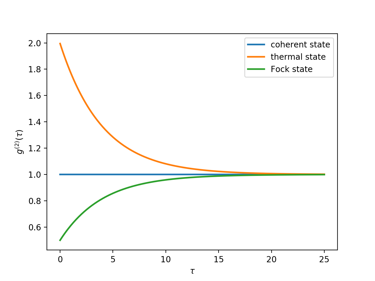
Example: second-order optical coherence function
The second-order optical coherence function, with time-delay \(\tau\), is defined as
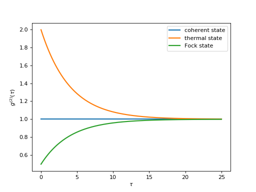
For a coherent state \(g^{(2)}(\tau) = 1\), for a thermal state \(g^{(2)}(\tau=0) = 2\) and it decreases as a function of time (bunched photons, they tend to appear together), and for a Fock state with \(n\) photons \(g^{(2)}(\tau = 0) = n(n - 1)/n^2 < 1\) and it increases with time (anti-bunched photons, more likely to arrive separated in time).
To calculate this type of correlation function with QuTiP, we can use qutip.correlation.correlation_4op_1t, which computes a correlation function on the form \(\left<A(0)B(\tau)C(\tau)D(0)\right>\) (four operators, one delay-time vector).
The following code calculates and plots \(g^{(2)}(\tau)\) as a function of \(\tau\) for a coherent, thermal and fock state.
import numpy as np
import pylab as plt
from qutip import *

N = 25
taus = np.linspace(0, 25.0, 200)
a = destroy(N)
H = 2 * np.pi * a.dag() * a

kappa = 0.25
n_th = 2.0  # bath temperature in terms of excitation number
c_ops = [np.sqrt(kappa * (1 + n_th)) * a, np.sqrt(kappa * n_th) * a.dag()]

states = [{'state': coherent_dm(N, np.sqrt(2)), 'label': "coherent state"},
          {'state': thermal_dm(N, 2), 'label': "thermal state"},
          {'state': fock_dm(N, 2), 'label': "Fock state"}]

fig, ax = plt.subplots(1, 1)

for state in states:
    rho0 = state['state']

    # first calculate the occupation number as a function of time
    n = mesolve(H, rho0, taus, c_ops, [a.dag() * a]).expect[0]

    # calculate the correlation function G2 and normalize with n(0)n(t) to
    # obtain g2
    G2 = correlation_3op_1t(H, rho0, taus, c_ops, a.dag(), a.dag()*a, a)
    g2 = G2 / (n[0] * n)

    ax.plot(taus, np.real(g2), label=state['label'], lw=2)

ax.legend(loc=0)
ax.set_xlabel(r'$\tau$')
ax.set_ylabel(r'$g^{(2)}(\tau)$')
plt.show()
(Source code, png, hires.png, pdf)
For convenience, the steps for calculating the second-order coherence function have been collected in the function qutip.correlation.coherence_function_g2.