Basic Operations on Quantum Objects
First things first
Important
Do not run QuTiP from the installation directory.
To load the qutip modules, we must first call the import statement:
In [1]: from qutip import *
that will load all of the user available functions. Often, we also need to import the Numpy and Matplotlib libraries with:
In [2]: import numpy as np
Note that, in the rest of the documentation, functions are written using qutip.module.function() notation which links to the corresponding function in the QuTiP API: Functions. However, in calling import *, we have already loaded all of the QuTiP modules. Therefore, we will only need the function name and not the complete path when calling the function from the interpreter prompt or a Python script.
The quantum object class
Introduction
The key difference between classical and quantum mechanics lies in the use of operators instead of numbers as variables. Moreover, we need to specify state vectors and their properties. Therefore, in computing the dynamics of quantum systems we need a data structure that is capable of encapsulating the properties of a quantum operator and ket/bra vectors. The quantum object class, qutip.Qobj, accomplishes this using matrix representation.
To begin, let us create a blank Qobj:
In [3]: Qobj()
Out[3]:
Quantum object: dims = [[1], [1]], shape = [1, 1], type = oper, isherm = True
Qobj data =
[[ 0.]]
where we see the blank `Qobj` object with dimensions, shape, and data. Here the data corresponds to a 1x1-dimensional matrix consisting of a single zero entry.
Hint
By convention, Class objects in Python such as Qobj() differ from functions in the use of a beginning capital letter.
We can create a Qobj with a user defined data set by passing a list or array of data into the Qobj:
In [4]: Qobj([1,2,3,4,5])
Out[4]:
Quantum object: dims = [[5], [1]], shape = [5, 1], type = ket
Qobj data =
[[ 1.]
 [ 2.]
 [ 3.]
 [ 4.]
 [ 5.]]

In [5]: x = array([[1, 2, 3, 4, 5]])

In [6]: Qobj(x)
Out[6]:
Quantum object: dims = [[1], [5]], shape = [1, 5], type = bra
Qobj data =
[[ 1.  2.  3.  4.  5.]]

In [7]: r = np.random.rand(4, 4)

In [8]: Qobj(r)
Out[8]:
Quantum object: dims = [[4], [4]], shape = [4, 4], type = oper, isherm = False
Qobj data =
[[ 0.53687843  0.03179873  0.29785873  0.04462891]
 [ 0.67900829  0.37491091  0.13618856  0.62680971]
 [ 0.41240537  0.50347257  0.26573402  0.2244419 ]
 [ 0.35279373  0.56183588  0.91221813  0.33800095]]
Notice how both the dims and shape change according to the input data. Although dims and shape appear to have the same function, the difference will become quite clear in the section on tensor products and partial traces.
Note
If you are running QuTiP from a python script you must use the print function to view the Qobj attributes.
States and operators
Manually specifying the data for each quantum object is inefficient. Even more so when most objects correspond to commonly used types such as the ladder operators of a harmonic oscillator, the Pauli spin operators for a two-level system, or state vectors such as Fock states. Therefore, QuTiP includes predefined objects for a variety of states:
| States | Command (# means optional) | Inputs |
|---|---|---|
| Fock state ket vector | basis(N,#m) / fock(N,#m) | N = number of levels in Hilbert space, m = level containing excitation (0 if no m given) |
| Fock density matrix (outer product of basis) | fock_dm(N,#p) | same as basis(N,m) / fock(N,m) |
| Coherent state | coherent(N,alpha) | alpha = complex number (eigenvalue) for requested coherent state |
| Coherent density matrix (outer product) | coherent_dm(N,alpha) | same as coherent(N,alpha) |
| Thermal density matrix (for n particles) | thermal_dm(N,n) | n = particle number expectation value |
and operators:
| Operators | Command (# means optional) | Inputs |
|---|---|---|
| Identity | qeye(N) | N = number of levels in Hilbert space. |
| Lowering (destruction) operator | destroy(N) | same as above |
| Raising (creation) operator | create(N) | same as above |
| Number operator | num(N) | same as above |
| Single-mode displacement operator | displace(N,alpha) | N=number of levels in Hilbert space, alpha = complex displacement amplitude. |
| Single-mode squeezing operator | squeez(N,sp) | N=number of levels in Hilbert space, sp = squeezing parameter. |
| Sigma-X | sigmax() | |
| Sigma-Y | sigmay() | |
| Sigma-Z | sigmaz() | |
| Sigma plus | sigmap() | |
| Sigma minus | sigmam() | |
| Higher spin operators | jmat(j,#s) | j = integer or half-integer representing spin, s = ‘x’, ‘y’, ‘z’, ‘+’, or ‘-‘ |
As an example, we give the output for a few of these functions:
In [9]: basis(5,3)
Out[9]:
Quantum object: dims = [[5], [1]], shape = [5, 1], type = ket
Qobj data =
[[ 0.]
 [ 0.]
 [ 0.]
 [ 1.]
 [ 0.]]

In [10]: coherent(5,0.5-0.5j)
Out[10]:
Quantum object: dims = [[5], [1]], shape = [5, 1], type = ket
Qobj data =
[[ 0.77880170+0.j        ]
 [ 0.38939142-0.38939142j]
 [ 0.00000000-0.27545895j]
 [-0.07898617-0.07898617j]
 [-0.04314271+0.j        ]]

In [11]: destroy(4)
Out[11]:
Quantum object: dims = [[4], [4]], shape = [4, 4], type = oper, isherm = False
Qobj data =
[[ 0.          1.          0.          0.        ]
 [ 0.          0.          1.41421356  0.        ]
 [ 0.          0.          0.          1.73205081]
 [ 0.          0.          0.          0.        ]]

In [12]: sigmaz()
Out[12]:
Quantum object: dims = [[2], [2]], shape = [2, 2], type = oper, isherm = True
Qobj data =
[[ 1.  0.]
 [ 0. -1.]]

In [13]: jmat(5/2.0,'+')
Out[13]:
Quantum object: dims = [[6], [6]], shape = [6, 6], type = oper, isherm = False
Qobj data =
[[ 0.          2.23606798  0.          0.          0.          0.        ]
 [ 0.          0.          2.82842712  0.          0.          0.        ]
 [ 0.          0.          0.          3.          0.          0.        ]
 [ 0.          0.          0.          0.          2.82842712  0.        ]
 [ 0.          0.          0.          0.          0.          2.23606798]
 [ 0.          0.          0.          0.          0.          0.        ]]
Qobj attributes
We have seen that a quantum object has several internal attributes, such as data, dims, and shape. These can be accessed in the following way:
In [14]: q = destroy(4)

In [15]: q.dims
Out[15]: [[4], [4]]

In [16]: q.shape
Out[16]: [4, 4]
In general, the attributes (properties) of a Qobj object (or any Python class) can be retrieved using the Q.attribute notation. In addition to the attributes shown with the print function, the Qobj class also has the following:
| Property | Attribute | Description |
|---|---|---|
| Data | Q.data | Matrix representing state or operator |
| Dimensions | Q.dims | List keeping track of shapes for individual components of a multipartite system (for tensor products and partial traces). |
| Shape | Q.shape | Dimensions of underlying data matrix. |
| is Hermitian? | Q.isherm | Is the operator Hermitian or not? |
| Type | Q.type | Is object of type ‘ket, ‘bra’, ‘oper’, or ‘super’? |
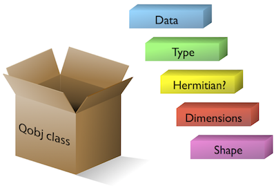
The Qobj Class viewed as a container for the properties need to characterize a quantum operator or state vector.
For the destruction operator above:
In [17]: q.type
Out[17]: 'oper'

In [18]: q.isherm
Out[18]: False

In [19]: q.data
Out[19]:
<4x4 sparse matrix of type '<type 'numpy.complex128'>'
	with 3 stored elements in Compressed Sparse Row format>
The data attribute returns a message stating that the data is a sparse matrix. All Qobj instances store their data as a sparse matrix to save memory. To access the underlying dense matrix one needs to use the qutip.Qobj.full function as described below.
Qobj Math
The rules for mathematical operations on Qobj instances are similar to standard matrix arithmetic:
In [20]: q = destroy(4)

In [21]: x = sigmax()

In [22]: q + 5
Out[22]:
Quantum object: dims = [[4], [4]], shape = [4, 4], type = oper, isherm = False
Qobj data =
[[ 5.          1.          0.          0.        ]
 [ 0.          5.          1.41421356  0.        ]
 [ 0.          0.          5.          1.73205081]
 [ 0.          0.          0.          5.        ]]

In [23]: x * x
Out[23]:
Quantum object: dims = [[2], [2]], shape = [2, 2], type = oper, isherm = True
Qobj data =
[[ 1.  0.]
 [ 0.  1.]]

In [24]: q ** 3
Out[24]:
Quantum object: dims = [[4], [4]], shape = [4, 4], type = oper, isherm = False
Qobj data =
[[ 0.          0.          0.          2.44948974]
 [ 0.          0.          0.          0.        ]
 [ 0.          0.          0.          0.        ]
 [ 0.          0.          0.          0.        ]]

In [25]: x / sqrt(2)
Out[25]:
Quantum object: dims = [[2], [2]], shape = [2, 2], type = oper, isherm = True
Qobj data =
[[ 0.          0.70710678]
 [ 0.70710678  0.        ]]
Of course, like matrices, multiplying two objects of incompatible shape throws an error:
>>> q * x
TypeError: Incompatible Qobj shapes
In addition, the logic operators is equal == and is not equal != are also supported.
Functions operating on Qobj class
Like attributes, the quantum object class has defined functions (methods) that operate on Qobj class instances. For a general quantum object Q:
| Function | Command | Description |
|---|---|---|
| Conjugate | Q.conj() | Conjugate of quantum object. |
| Dagger (adjoint) | Q.dag() | Returns adjoint (dagger) of object. |
| Diagonal | Q.diag() | Returns the diagonal elements. |
| Eigenenergies | Q.eigenenergies() | Eigenenergies (values) of operator. |
| Eigenstates | Q.eigenstates() | Returns eigenvalues and eigenvectors. |
| Exponential | Q.expm() | Matrix exponential of operator. |
| Full | Q.full() | Returns full (not sparse) array of Q’s data. |
| Groundstate | Q.groundstate() | Eigenval & eigket of Qobj groundstate. |
| Matrix Element | Q.matrix_element(bra,ket) | Matrix element <bra|Q|ket> |
| Norm | Q.norm() | Returns L2 norm for states, trace norm for operators. |
| Partial Trace | Q.ptrace(sel) | Partial trace returning components selected using ‘sel’ parameter. |
| Permute | Q.permute(order) | Permutes the tensor structure of a composite object in the given order. |
| Sqrt | Q.sqrtm() | Matrix sqrt of operator. |
| Tidyup | Q.tidyup() | Removes small elements from Qobj. |
| Trace | Q.tr() | Returns trace of quantum object. |
| Transform | Q.transform(inpt) | A basis transformation defined by matrix or list of kets ‘inpt’ . |
| Transpose | Q.trans() | Transpose of quantum object. |
| Unit | Q.unit() | Returns normalized (unit) vector Q/Q.norm(). |
In [26]: basis(5, 3)
Out[26]:
Quantum object: dims = [[5], [1]], shape = [5, 1], type = ket
Qobj data =
[[ 0.]
 [ 0.]
 [ 0.]
 [ 1.]
 [ 0.]]

In [27]: basis(5, 3).dag()
Out[27]:
Quantum object: dims = [[1], [5]], shape = [1, 5], type = bra
Qobj data =
[[ 0.  0.  0.  1.  0.]]

In [28]: coherent_dm(5, 1)
Out[28]:
Quantum object: dims = [[5], [5]], shape = [5, 5], type = oper, isherm = True
Qobj data =
[[ 0.36791117  0.36774407  0.26105441  0.14620658  0.08826704]
 [ 0.36774407  0.36757705  0.26093584  0.14614018  0.08822695]
 [ 0.26105441  0.26093584  0.18523331  0.10374209  0.06263061]
 [ 0.14620658  0.14614018  0.10374209  0.05810197  0.035077  ]
 [ 0.08826704  0.08822695  0.06263061  0.035077    0.0211765 ]]

In [29]: coherent_dm(5, 1).diag()
Out[29]: array([ 0.36791117,  0.36757705,  0.18523331,  0.05810197,  0.0211765 ])

In [30]: coherent_dm(5, 1).full()
Out[30]:
array([[ 0.36791117+0.j,  0.36774407+0.j,  0.26105441+0.j,  0.14620658+0.j,
         0.08826704+0.j],
       [ 0.36774407+0.j,  0.36757705+0.j,  0.26093584+0.j,  0.14614018+0.j,
         0.08822695+0.j],
       [ 0.26105441+0.j,  0.26093584+0.j,  0.18523331+0.j,  0.10374209+0.j,
         0.06263061+0.j],
       [ 0.14620658+0.j,  0.14614018+0.j,  0.10374209+0.j,  0.05810197+0.j,
         0.03507700+0.j],
       [ 0.08826704+0.j,  0.08822695+0.j,  0.06263061+0.j,  0.03507700+0.j,
         0.02117650+0.j]])

In [31]: coherent_dm(5, 1).norm()
Out[31]: 1.0000000000000002

In [32]: coherent_dm(5, 1).sqrtm()
Out[32]:
Quantum object: dims = [[5], [5]], shape = [5, 5], type = oper, isherm = False
Qobj data =
[[ 0.36791119 +0.00000000e+00j  0.36774406 +0.00000000e+00j
   0.26105440 +0.00000000e+00j  0.14620658 +0.00000000e+00j
   0.08826704 +0.00000000e+00j]
 [ 0.36774406 +0.00000000e+00j  0.36757705 +4.97355349e-13j
   0.26093584 -4.95568446e-12j  0.14614018 -4.38433154e-12j
   0.08822695 +1.98468419e-11j]
 [ 0.26105440 +0.00000000e+00j  0.26093584 -4.95568446e-12j
   0.18523332 +4.93787964e-11j  0.10374209 +4.36857948e-11j
   0.06263061 -1.97755360e-10j]
 [ 0.14620658 +0.00000000e+00j  0.14614018 -4.38433154e-12j
   0.10374209 +4.36857948e-11j  0.05810197 +3.86491532e-11j
   0.03507701 -1.74955663e-10j]
 [ 0.08826704 +0.00000000e+00j  0.08822695 +1.98468419e-11j
   0.06263061 -1.97755360e-10j  0.03507701 -1.74955663e-10j
   0.02117650 +7.91983303e-10j]]

In [33]: coherent_dm(5, 1).tr()
Out[33]: 1.0

In [34]: (basis(4, 2) + basis(4, 1)).unit()
Out[34]:
Quantum object: dims = [[4], [1]], shape = [4, 1], type = ket
Qobj data =
[[ 0.        ]
 [ 0.70710678]
 [ 0.70710678]
 [ 0.        ]]