Arbitrary Precision

Double precision (Float64) carries about 16 significant decimal digits. For the overwhelming majority of quantum simulations that is far more than enough, and you should keep using it.

But some of the most interesting quantities in quantum physics are exponentially small: tunneling splittings, Liouvillian gaps, metastable switching rates, and the lifetimes of symmetry-broken states all scale like for some action or system size . Push a little deeper into the parameter regime and the number you are chasing drops below relative to the energy scales in your Hamiltonian. At that point the answer is no longer physics — it is roundoff.

The failure is quiet, which is what makes it dangerous. The eigensolver still converges, the numbers still look plausible, and the plot still has a curve on it. It is simply the wrong curve. Below we show an example where Float64 confidently reports a result that is wrong by nearly ten orders of magnitude, and where switching a single type argument fixes it.

QuantumToolbox.jl supports arbitrary precision throughout: states, operators, superoperators, the eigensolvers, and the time-evolution solvers are all generic over the number type.

Why Julia makes this possible

This capability is not something QuantumToolbox.jl implements by hand — it is inherited from Julia's generic programming model, in the same way that Automatic Differentiation support was largely inherited rather than built.

Julia compiles the same generic source code into specialized native code for whichever number type you hand it. destroy(Complex{BigFloat}, N) does not run a separate high-precision code path; it runs the same one, respecialized by the compiler for Complex{BigFloat}. Nothing in the library needs to know in advance which types users will care about.

It is worth being precise about why this is hard elsewhere:

• Python QuTiP cannot do this at all. Its data layer (Dense and CSR) is compiled Cython with double complex hardcoded, so precision is not a knob that exists.

• JAX cannot either. XLA supports only hardware float types (bf16, f16, f32, f64); arbitrary precision has nowhere to compile to.

• NumPy technically can, via dtype=object arrays holding mpmath scalars, but every elementary operation then becomes an interpreted per-element Python call with no BLAS behind it — a fundamentally different and far slower execution path than the fast one.

The honest caveat is that BigFloat is not magic: it wraps the MPFR C library, allocates on the heap, and is genuinely slow. The more interesting part of the story is types like Double64 from DoubleFloats.jl, which represents ~32 digits as a pair of Float64s. It is written in pure Julia, so it inlines and compiles down to ordinary floating-point instructions with no interpreter overhead at all — while remaining a type the library has never heard of. That combination is what Python and JAX structurally cannot offer.

A warm-up: where double precision runs out

Before touching quantum objects, it helps to see the mechanism in isolation. Consider evaluating   for large . For   the two square roots agree to ~16 digits, so subtracting them cancels away every digit you had — this is catastrophic cancellation. The algebraically identical form

never subtracts nearby numbers, and so is stable.

using DoubleFloats

setprecision(BigFloat, 256)

naive(x) = sqrt(x + 1) - sqrt(x)
stable(x) = 1 / (sqrt(x + 1) + sqrt(x))

reference = stable(BigFloat("1e16"))   # 256-bit reference value

for (label, x) in (
    ("Float64 ", 1e16),
    ("Double64", Double64("1e16")),
    ("BigFloat", BigFloat("1e16")),
)
    err(v) = Float64(abs((BigFloat(v) - reference) / reference))
    println("$label   naive: ", rpad(Float64(naive(x)), 24), " (rel. err. ", err(naive(x)), ")")
    println("$label  stable: ", rpad(Float64(stable(x)), 24), " (rel. err. ", err(stable(x)), ")")
end

Float64    naive: 0.0                      (rel. err. 1.0)
Float64   stable: 5.0e-9                   (rel. err. 4.592256083012847e-17)
Double64   naive: 5.0e-9                   (rel. err. 4.592256083012847e-17)
Double64  stable: 5.0e-9                   (rel. err. 2.351648722519036e-33)
BigFloat   naive: 5.0e-9                   (rel. err. 6.800699326188808e-63)
BigFloat  stable: 5.0e-9                   (rel. err. 0.0)

Float64 with the naive formula returns exactly zero: not an inaccurate answer, but a complete loss of every significant digit. Note the two independent levers here — a better algorithm (the stable formula) and a better number type. Extra precision is not a substitute for numerical care, and the rest of this page is about the cases where care alone is not enough.

Using arbitrary precision in QuantumToolbox

Every state and operator generating function takes an optional leading argument for specifying element type:

using QuantumToolbox

destroy(Complex{BigFloat}, 5)

Quantum Object:   type=Operator()   dims=([5], [5])   size=(5, 5)   ishermitian=false
5×5 SparseArrays.SparseMatrixCSC{Complex{BigFloat}, Int64} with 4 stored entries:
     ⋅      1.0+0.0im          ⋅              ⋅          ⋅    
     ⋅          ⋅      1.41421+0.0im          ⋅          ⋅    
     ⋅          ⋅              ⋅      1.73205+0.0im      ⋅    
     ⋅          ⋅              ⋅              ⋅      2.0+0.0im
     ⋅          ⋅              ⋅              ⋅          ⋅

which propagates through arithmetic exactly as you would expect:

normalize(fock(BigFloat, 10, 3) + fock(BigFloat, 10, 4))

Quantum Object:   type=Ket()   dims=([10], [1])   size=(10,)
10-element Vector{BigFloat}:
 0.0
 0.0
 0.0
 0.7071067811865475244008443621048490392848359376884740365883398689953662392310596
 0.7071067811865475244008443621048490392848359376884740365883398689953662392310596
 0.0
 0.0
 0.0
 0.0
 0.0

Some functions instead infer the element type from the value you pass, which is often more convenient:

α = BigFloat(1) + 1im * BigFloat(1)
coherent(6, α)   # eltype follows α

Quantum Object:   type=Ket()   dims=([6], [1])   size=(6,)
6-element Vector{Complex{BigFloat}}:
  0.3678194156604567805609171083785753670208413923411958333483643334244848527851409 + 0.0im
  0.3682113270926567801078591727881763306620827870825117172415432286616889759048283 + 0.3682113270926567801078591727881763306620827870825117172415432286616889759048283im
                                                                                0.0 + 0.5178970835307337693350190087849629951639584815571087371895738598509131809743191im
 -0.3065807830506954336610335662446692550238719459912961269919298182151938479866725 + 0.3065807830506954336610335662446692550238719459912961269919298182151938479866725im
 -0.2750166810074569578245828199003319722932577714756162298307816555463210731490361 + 0.0im
 -0.1756624570455748194555105240056445098801022584838696287887496604888957283194441 - 0.1756624570455748194555105240056445098801022584838696287887496604888957283194441im

The working precision of BigFloat is global and set with setprecision (in bits — 128 bits is ~38 decimal digits, and is usually plenty):

setprecision(BigFloat, 128)
eltype(destroy(Complex{BigFloat}, 5))

Complex{BigFloat}

Which packages do I need?

Core operations work out of the box, but the eigensolvers need generic linear algebra backends that are not QuantumToolbox.jl dependencies. Load them yourself:

• GenericSchur.jl — the generic Schur decomposition used by eigenstates and eigsolve for non-BlasFloat element types.

• Sparspak.jl — generic sparse LU, needed for the sparse shift-and-invert path (sparse = Val(true) with a sigma).

• DoubleFloats.jl — optional, provides Double64.

Forgetting these produces a MethodError from LinearAlgebra, not an obvious "unsupported precision" message.

Exponentially small tunneling splittings

Now the physics. Take a particle in a quartic double well (in units    ),

with minima at    separated by a barrier of height . The two lowest eigenstates are the symmetric and antisymmetric combinations of the states localized in each well, and they are split by an energy    that is exponentially small in the barrier action. That splitting is the entire physics of the problem: a particle prepared in the left well tunnels to the right one in a time .

We build and from the annihilation operator, so that the whole Hamiltonian inherits whatever type we pass in:

using LinearAlgebra
using GenericSchur   # generic Schur decomposition, needed for non-Float64 eigensolvers

function double_well(::Type{T}, N, λ, x0) where {T}
    a = destroy(T, N)
    x = (a' + a) / sqrt(T(2))
    p = im * (a' - a) / sqrt(T(2))
    W = x * x - T(x0)^2 * qeye(T, N)
    return p * p / 2 + T(λ) * W * W
end

# splitting between the two lowest levels
function splitting(::Type{T}, N, λ, x0) where {T}
    E = real.(eigenstates(double_well(T, N, λ, x0)).values)
    return E[2] - E[1]
end

Note that double_well contains no reference to precision whatsoever — it is ordinary code, written the way you would write it anyway. Now sweep the well separation (deepening the barrier) at three different precisions:

N = 250     # Fock cutoff, large enough to be converged at the deepest barrier
λ = 0.5
x0_list = range(1.0, 3.5, 11)

Δ64  = [splitting(ComplexF64, N, λ, x0) for x0 in x0_list]
Δd64 = [splitting(Complex{Double64}, N, λ, x0) for x0 in x0_list]

# cross-check the deepest barrier against BigFloat (much slower, so just one point)
Δbig_end = splitting(Complex{BigFloat}, N, λ, x0_list[end])

println("at the deepest barrier, x0 = ", x0_list[end])
println("  Float64  : ", Δ64[end])
println("  Double64 : ", Δd64[end])
println("  BigFloat : ", Δbig_end)

at the deepest barrier, x0 = 3.5
  Float64  : 6.217248937900877e-15
  Double64 : 2.1385342840226823e-23
  BigFloat : 2.138512717325345574943810883191401066627e-23

Float64 reports a splitting of while the true value is — wrong by nearly ten orders of magnitude. Double64 already agrees with BigFloat to several digits here, so the cheap type is enough and we can plot it alone. Sweeping the whole range shows how the failure sets in:

using CairoMakie
CairoMakie.enable_only_mime!(MIME"image/svg+xml"())

fig = Figure(size = (600, 400))
ax = Axis(fig[1, 1],
    title = "Tunneling splitting of a quartic double well",
    xlabel = L"well separation $x_0$",
    ylabel = L"\Delta E = E_1 - E_0",
    yscale = log10,
)
lines!(ax, x0_list, abs.(Δ64), label = "Float64", linewidth = 2)
lines!(ax, x0_list, abs.(Float64.(Δd64)), label = "Double64", linewidth = 2, linestyle = :dash)
axislegend(ax, position = :lb)

fig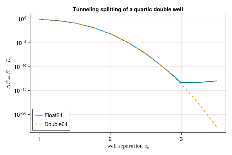

The two curves agree perfectly while the splitting is large. Around   the Float64 curve simply stops descending and flattens into a noise floor, wandering non-monotonically from point to point — it is now reporting the accumulated roundoff of the eigensolver rather than a physical energy. Double64 continues down the straight line that the exponential law predicts.

Read physically, the Float64 curve claims that beyond   the barrier stops mattering and the tunneling rate saturates. That is not a small quantitative error; it is a qualitatively wrong statement about the system. Tunneling keeps slowing down exponentially, and only the high-precision types can see it.

The same trap appears in open systems. The Liouvillian gap of a driven-dissipative resonator — the eigenvalue of with the smallest nonzero real part, which sets the switching time between metastable states — becomes exponentially small near a bistability, and shrinks further with system size. Computed in Float64 it eventually stops being physics: it flattens into the same roundoff floor, can come out negative (implying a density matrix that grows without bound, which no Lindblad master equation permits), and can place the gap minimum at entirely the wrong drive amplitude. The remedy is identical — pass a wider element type to liouvillian and eigenstates.

Note also that Double64, not BigFloat, was enough here, at roughly a tenth of the cost. Reaching for BigFloat on every problem is rarely the right move; it is usually worth trying the cheap type first.

The solvers are generic too

The same type argument flows through the time-evolution solvers, so sesolve and mesolve work unchanged at high precision:

N_solver = 20
a_big = destroy(Complex{BigFloat}, N_solver)
ψ0_big = fock(Complex{BigFloat}, N_solver, 1)
H_big = a_big' * a_big + BigFloat(0.1) / 2 * a_big' * a_big' * a_big * a_big
c_ops_big = [sqrt(BigFloat(0.1)) * a_big]

tlist = range(0, 10, 100)
sol = mesolve(H_big, ψ0_big, tlist, c_ops_big, e_ops = [a_big' * a_big], progress_bar = Val(false))

eltype(sol.expect)

Complex{BigFloat}

Note that the expectation values come back in the element type you asked for, rather than being silently narrowed to ComplexF64.

Be aware of what this does and does not buy you. Extra precision does not generally make a time-evolution result better: the error of an ODE integration is dominated by the solver tolerances, not by roundoff, and tightening abstol/reltol in Float64 is both cheaper and more effective. High-precision solvers earn their cost when the evolution feeds something else that is precision-critical — for example eigsolve_al, which integrates the master equation to extract Liouvillian eigenvalues, and so inherits exactly the sensitivity described above.

Caveats and performance

Arbitrary precision is not free

• It is slow. BigFloat allocates on the heap and calls into MPFR for every operation; expect one to two orders of magnitude slowdown, and no multithreaded BLAS. Double64 is typically only a few times slower than Float64 and should be your first try — in the double-well sweep above it is roughly ten times faster than BigFloat and gives an identical answer.

• No GPU support. The CUDA extension deliberately supports only Float32/Float64 word sizes; arbitrary precision is CPU-only.

• Convergence is not just about precision. In the double-well example the Fock cutoff N must be large enough that the truncated problem is converged. At N = 150, even BigFloat returns a wrong splitting — the arithmetic is exact but the basis is not. Increasing precision cannot fix a basis-truncation error, so check both.

• Tolerances do not scale automatically. eigsolve's default tol = 1e-8 is a hardcoded Float64 literal. If you want more digits than that out of an iterative solver, pass a tighter tol explicitly.

• Tested surface. Arbitrary precision is covered by the test suite for sesolve, mesolve, eigenstates, and eigsolve_al. Other routines such as steadystate, mcsolve, and spectrum are written generically and may well work, but are not currently tested at high precision — if you rely on them, validate against a Float64 result in a regime where both are trustworthy.