Lindblad Master Equation Solver¶

Unitary evolution¶

The dynamics of a closed (pure) quantum system is governed by the Schrödinger equation

where \(\Psi\) is the wave function, \(\hat H\) the Hamiltonian, and \(\hbar\) is Planck’s constant. In general, the Schrödinger equation is a partial differential equation (PDE) where both \(\Psi\) and \(\hat H\) are functions of space and time. For computational purposes it is useful to expand the PDE in a set of basis functions that span the Hilbert space of the Hamiltonian, and to write the equation in matrix and vector form

where \(\left|\psi\right>\) is the state vector and \(H\) is the matrix representation of the Hamiltonian. This matrix equation can, in principle, be solved by diagonalizing the Hamiltonian matrix \(H\). In practice, however, it is difficult to perform this diagonalization unless the size of the Hilbert space (dimension of the matrix \(H\)) is small. Analytically, it is a formidable task to calculate the dynamics for systems with more than two states. If, in addition, we consider dissipation due to the inevitable interaction with a surrounding environment, the computational complexity grows even larger, and we have to resort to numerical calculations in all realistic situations. This illustrates the importance of numerical calculations in describing the dynamics of open quantum systems, and the need for efficient and accessible tools for this task.

The Schrödinger equation, which governs the time-evolution of closed quantum systems, is defined by its Hamiltonian and state vector. In the previous section, Using Tensor Products and Partial Traces, we showed how Hamiltonians and state vectors are constructed in QuTiP. Given a Hamiltonian, we can calculate the unitary (non-dissipative) time-evolution of an arbitrary state vector \(\left|\psi_0\right>\) (psi0) using the QuTiP function qutip.mesolve. It evolves the state vector and evaluates the expectation values for a set of operators expt_ops at the points in time in the list times, using an ordinary differential equation solver. Alternatively, we can use the function qutip.essolve, which uses the exponential-series technique to calculate the time evolution of a system. The qutip.mesolve and qutip.essolve functions take the same arguments and it is therefore easy switch between the two solvers.

For example, the time evolution of a quantum spin-1/2 system with tunneling rate 0.1 that initially is in the up state is calculated, and the expectation values of the \(\sigma_z\) operator evaluated, with the following code

In [1]: H = 2 * np.pi * 0.1 * sigmax()

In [2]: psi0 = basis(2, 0)

In [3]: times = np.linspace(0.0, 10.0, 20.0)

In [4]: result = mesolve(H, psi0, times, [], [sigmaz()])

The brackets in the fourth argument is an empty list of collapse operators, since we consider unitary evolution in this example. See the next section for examples on how dissipation is included by defining a list of collapse operators.

The function returns an instance of qutip.solver.Result, as described in the previous section Dynamics Simulation Results. The attribute expect in result is a list of expectation values for the operators that are included in the list in the fifth argument. Adding operators to this list results in a larger output list returned by the function (one array of numbers, corresponding to the times in times, for each operator)

In [5]: result = mesolve(H, psi0, times, [], [sigmaz(), sigmay()])

In [6]: result.expect
Out[6]: 
[array([ 1.        ,  0.78914057,  0.24548559, -0.40169513, -0.8794735 ,
        -0.98636142, -0.67728219, -0.08258023,  0.54694721,  0.94581685,
         0.94581769,  0.54694945, -0.08257765, -0.67728015, -0.98636097,
        -0.87947476, -0.40169736,  0.24548326,  0.78913896,  1.        ]),
 array([ 0.00000000e+00, -6.14212640e-01, -9.69400240e-01, -9.15773457e-01,
        -4.75947849e-01,  1.64593874e-01,  7.35723339e-01,  9.96584419e-01,
         8.37167094e-01,  3.24700624e-01, -3.24698160e-01, -8.37165632e-01,
        -9.96584633e-01, -7.35725221e-01, -1.64596567e-01,  4.75945525e-01,
         9.15772479e-01,  9.69400830e-01,  6.14214701e-01,  2.77159958e-06])]

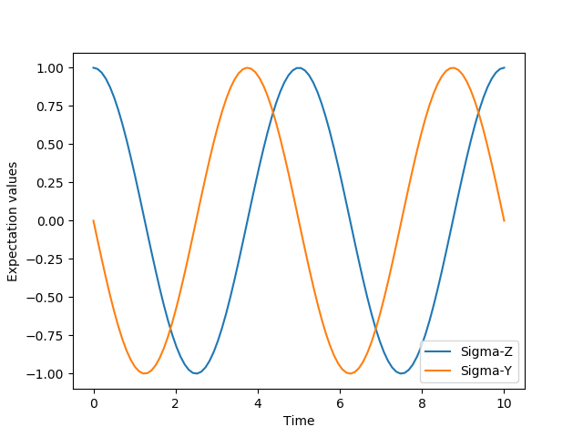
The resulting list of expectation values can easily be visualized using matplotlib’s plotting functions:

In [7]: H = 2 * np.pi * 0.1 * sigmax()

In [8]: psi0 = basis(2, 0)

In [9]: times = np.linspace(0.0, 10.0, 100)

In [10]: result = mesolve(H, psi0, times, [], [sigmaz(), sigmay()])

In [11]: fig, ax = subplots()

In [12]: ax.plot(result.times, result.expect[0]);

In [13]: ax.plot(result.times, result.expect[1]);

In [14]: ax.set_xlabel('Time');

In [15]: ax.set_ylabel('Expectation values');

In [16]: ax.legend(("Sigma-Z", "Sigma-Y"));

In [17]: show()

If an empty list of operators is passed as fifth parameter, the qutip.mesolve function returns a qutip.solver.Result instance that contains a list of state vectors for the times specified in times

In [18]: times = [0.0, 1.0]

In [19]: result = mesolve(H, psi0, times, [], [])

In [20]: result.states
Out[20]: 
[Quantum object: dims = [[2], [1]], shape = (2, 1), type = ket
 Qobj data =
 [[1.]
  [0.]], Quantum object: dims = [[2], [1]], shape = (2, 1), type = ket
 Qobj data =
 [[0.80901699+0.j        ]
  [0.        -0.58778526j]]]

Non-unitary evolution¶

While the evolution of the state vector in a closed quantum system is deterministic, open quantum systems are stochastic in nature. The effect of an environment on the system of interest is to induce stochastic transitions between energy levels, and to introduce uncertainty in the phase difference between states of the system. The state of an open quantum system is therefore described in terms of ensemble averaged states using the density matrix formalism. A density matrix \(\rho\) describes a probability distribution of quantum states \(\left|\psi_n\right>\), in a matrix representation \(\rho = \sum_n p_n \left|\psi_n\right>\left<\psi_n\right|\), where \(p_n\) is the classical probability that the system is in the quantum state \(\left|\psi_n\right>\). The time evolution of a density matrix \(\rho\) is the topic of the remaining portions of this section.

The Lindblad Master equation¶

The standard approach for deriving the equations of motion for a system interacting with its environment is to expand the scope of the system to include the environment. The combined quantum system is then closed, and its evolution is governed by the von Neumann equation

the equivalent of the Schrödinger equation (1) in the density matrix formalism. Here, the total Hamiltonian

includes the original system Hamiltonian \(H_{\rm sys}\), the Hamiltonian for the environment \(H_{\rm env}\), and a term representing the interaction between the system and its environment \(H_{\rm int}\). Since we are only interested in the dynamics of the system, we can at this point perform a partial trace over the environmental degrees of freedom in Eq. (2), and thereby obtain a master equation for the motion of the original system density matrix. The most general trace-preserving and completely positive form of this evolution is the Lindblad master equation for the reduced density matrix \(\rho = {\rm Tr}_{\rm env}[\rho_{\rm tot}]\)

where the \(C_n = \sqrt{\gamma_n} A_n\) are collapse operators, and \(A_n\) are the operators through which the environment couples to the system in \(H_{\rm int}\), and \(\gamma_n\) are the corresponding rates. The derivation of Eq. (3) may be found in several sources, and will not be reproduced here. Instead, we emphasize the approximations that are required to arrive at the master equation in the form of Eq. (3) from physical arguments, and hence perform a calculation in QuTiP:

• Separability: At \(t=0\) there are no correlations between the system and its environment such that the total density matrix can be written as a tensor product \(\rho^I_{\rm tot}(0) = \rho^I(0) \otimes \rho^I_{\rm env}(0)\).
• Born approximation: Requires: (1) that the state of the environment does not significantly change as a result of the interaction with the system; (2) The system and the environment remain separable throughout the evolution. These assumptions are justified if the interaction is weak, and if the environment is much larger than the system. In summary, \(\rho_{\rm tot}(t) \approx \rho(t)\otimes\rho_{\rm env}\).
• Markov approximation The time-scale of decay for the environment \(\tau_{\rm env}\) is much shorter than the smallest time-scale of the system dynamics \(\tau_{\rm sys} \gg \tau_{\rm env}\). This approximation is often deemed a “short-memory environment” as it requires that environmental correlation functions decay on a time-scale fast compared to those of the system.
• Secular approximation Stipulates that elements in the master equation corresponding to transition frequencies satisfy \(|\omega_{ab}-\omega_{cd}| \ll 1/\tau_{\rm sys}\), i.e., all fast rotating terms in the interaction picture can be neglected. It also ignores terms that lead to a small renormalization of the system energy levels. This approximation is not strictly necessary for all master-equation formalisms (e.g., the Block-Redfield master equation), but it is required for arriving at the Lindblad form (3) which is used in qutip.mesolve.

For systems with environments satisfying the conditions outlined above, the Lindblad master equation (3) governs the time-evolution of the system density matrix, giving an ensemble average of the system dynamics. In order to ensure that these approximations are not violated, it is important that the decay rates \(\gamma_n\) be smaller than the minimum energy splitting in the system Hamiltonian. Situations that demand special attention therefore include, for example, systems strongly coupled to their environment, and systems with degenerate or nearly degenerate energy levels.

For non-unitary evolution of a quantum systems, i.e., evolution that includes incoherent processes such as relaxation and dephasing, it is common to use master equations. In QuTiP, the same function (qutip.mesolve) is used for evolution both according to the Schrödinger equation and to the master equation, even though these two equations of motion are very different. The qutip.mesolve function automatically determines if it is sufficient to use the Schrödinger equation (if no collapse operators were given) or if it has to use the master equation (if collapse operators were given). Note that to calculate the time evolution according to the Schrödinger equation is easier and much faster (for large systems) than using the master equation, so if possible the solver will fall back on using the Schrödinger equation.

What is new in the master equation compared to the Schrödinger equation are processes that describe dissipation in the quantum system due to its interaction with an environment. These environmental interactions are defined by the operators through which the system couples to the environment, and rates that describe the strength of the processes.

In QuTiP, the product of the square root of the rate and the operator that describe the dissipation process is called a collapse operator. A list of collapse operators (c_ops) is passed as the fourth argument to the qutip.mesolve function in order to define the dissipation processes in the master equation. When the c_ops isn’t empty, the qutip.mesolve function will use the master equation instead of the unitary Schrödinger equation.

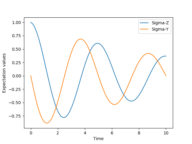
Using the example with the spin dynamics from the previous section, we can easily add a relaxation process (describing the dissipation of energy from the spin to its environment), by adding np.sqrt(0.05) * sigmax() to the previously empty list in the fourth parameter to the qutip.mesolve function:

In [21]: times = np.linspace(0.0, 10.0, 100)

In [22]: result = mesolve(H, psi0, times, [np.sqrt(0.05) * sigmax()], [sigmaz(), sigmay()])

In [23]: fig, ax = subplots()

In [24]: ax.plot(times, result.expect[0]);

In [25]: ax.plot(times, result.expect[1]);

In [26]: ax.set_xlabel('Time');

In [27]: ax.set_ylabel('Expectation values');

In [28]: ax.legend(("Sigma-Z", "Sigma-Y"));

In [29]: show(fig)

Here, 0.05 is the rate and the operator \(\sigma_x\) (qutip.operators.sigmax) describes the dissipation process.

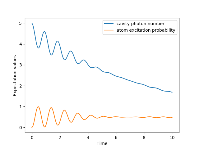
Now a slightly more complex example: Consider a two-level atom coupled to a leaky single-mode cavity through a dipole-type interaction, which supports a coherent exchange of quanta between the two systems. If the atom initially is in its groundstate and the cavity in a 5-photon Fock state, the dynamics is calculated with the lines following code

In [30]: times = np.linspace(0.0, 10.0, 200)

In [31]: psi0 = tensor(fock(2,0), fock(10, 5))

In [32]: a  = tensor(qeye(2), destroy(10))

In [33]: sm = tensor(destroy(2), qeye(10))

In [34]: H = 2 * np.pi * a.dag() * a + 2 * np.pi * sm.dag() * sm + \
   ....: 2 * np.pi * 0.25 * (sm * a.dag() + sm.dag() * a)
   ....: 

In [35]: result = mesolve(H, psi0, times, [np.sqrt(0.1)*a], [a.dag()*a, sm.dag()*sm])

In [36]: figure()
Out[36]: <Figure size 640x480 with 0 Axes>

In [37]: plot(times, result.expect[0])
Out[37]: [<matplotlib.lines.Line2D at 0x11772c4a8>]

In [38]: plot(times, result.expect[1])
Out[38]: [<matplotlib.lines.Line2D at 0x1a28aad5f8>]

In [39]: xlabel('Time')
Out[39]: Text(0.5,0,'Time')

In [40]: ylabel('Expectation values')
Out[40]: Text(0,0.5,'Expectation values')

In [41]: legend(("cavity photon number", "atom excitation probability"))
Out[41]: <matplotlib.legend.Legend at 0x1a27fef7f0>

In [42]: show()