Two-time correlation functions
With the QuTiP time-evolution functions (for example qutip.mesolve and qutip.mcsolve), a state vector or density matrix can be evolved from an initial state at \(t_0\) to an arbitrary time \(t\), \(\rho(t)=V(t, t_0)\left\{\rho(t_0)\right\}\), where \(V(t, t_0)\) is the propagator defined by the equation of motion. The resulting density matrix can then be used to evaluate the expectation values of arbitrary combinations of same-time operators.
To calculate two-time correlation functions on the form \(\left<A(t+\tau)B(t)\right>\), we can use the quantum regression theorem (see, e.g., [Gar03]) to write
We therefore first calculate \(\rho(t)=V(t, 0)\left\{\rho(0)\right\}\) using one of the QuTiP evolution solvers with \(\rho(0)\) as initial state, and then again use the same solver to calculate \(V(t+\tau, t)\left\{B\rho(t)\right\}\) using \(B\rho(t)\) as initial state.
Note that if the intial state is the steady state, then \(\rho(t)=V(t, 0)\left\{\rho_{\rm ss}\right\}=\rho_{\rm ss}\) and
which is independent of \(t\), so that we only have one time coordinate \(\tau\).
QuTiP provides a family of functions that assists in the process of calculating two-time correlation functions. The available functions and their usage is show in the table below. Each of these functions can use one of the following evolution solvers: Master-equation, Exponential series and the Monte-Carlo. The choice of solver is defined by the optional argument solver.
| QuTiP function | Correlation function |
|---|---|
| qutip.correlation.correlation or qutip.correlation.correlation_2op_2t | \(\left<A(t+\tau)B(t)\right>\) or \(\left<A(t)B(t+\tau)\right>\). |
| qutip.correlation.correlation_ss or qutip.correlation.correlation_2op_1t | \(\left<A(\tau)B(0)\right>\) or \(\left<A(0)B(\tau)\right>\). |
| qutip.correlation.correlation_4op_1t | \(\left<A(0)B(\tau)C(\tau)D(0)\right>\). |
| qutip.correlation.correlation_4op_2t | \(\left<A(t)B(t+\tau)C(t+\tau)D(t)\right>\). |
The most common use-case is to calculate correlation functions of the kind \(\left<A(\tau)B(0)\right>\), in which case we use the correlation function solvers that start from the steady state, e.g., the qutip.correlation.correlation_2op_1t function. These correlation function sovlers return a vector or matrix (in general complex) with the correlations as a function of the delays times.
Steadystate correlation function
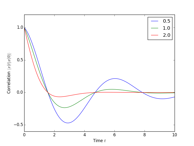
The following code demonstrates how to calculate the \(\left<x(t)x(0)\right>\) correlation for a leaky cavity with three different relaxation rates.
In [1]: times = np.linspace(0,10.0,200)

In [2]: a = destroy(10)

In [3]: x = a.dag() + a

In [4]: H = a.dag() * a

In [5]: corr1 = correlation_ss(H, times, [np.sqrt(0.5) * a], x, x)

In [6]: corr2 = correlation_ss(H, times, [np.sqrt(1.0) * a], x, x)

In [7]: corr3 = correlation_ss(H, times, [np.sqrt(2.0) * a], x, x)

In [8]: figure()
Out[8]: <matplotlib.figure.Figure at 0x10b2196d0>

In [9]: plot(times, np.real(corr1), times, np.real(corr2), times, np.real(corr3))
Out[9]:
[<matplotlib.lines.Line2D at 0x10b4a3490>,
 <matplotlib.lines.Line2D at 0x10b4a33d0>,
 <matplotlib.lines.Line2D at 0x10b4fddd0>]

In [10]: legend(['0.5','1.0','2.0'])
Out[10]: <matplotlib.legend.Legend at 0x10df0d310>

In [11]: xlabel(r'Time $t$')
Out[11]: <matplotlib.text.Text at 0x10d29b1d0>

In [12]: ylabel(r'Correlation $\left<x(t)x(0)\right>$')
Out[12]: <matplotlib.text.Text at 0x10d263f90>

In [13]: show()
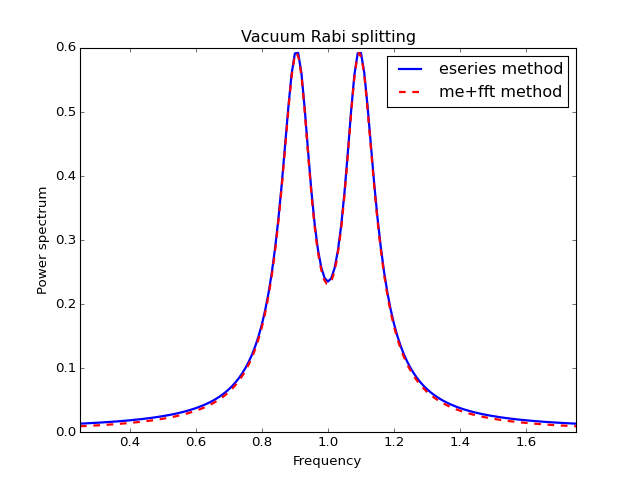
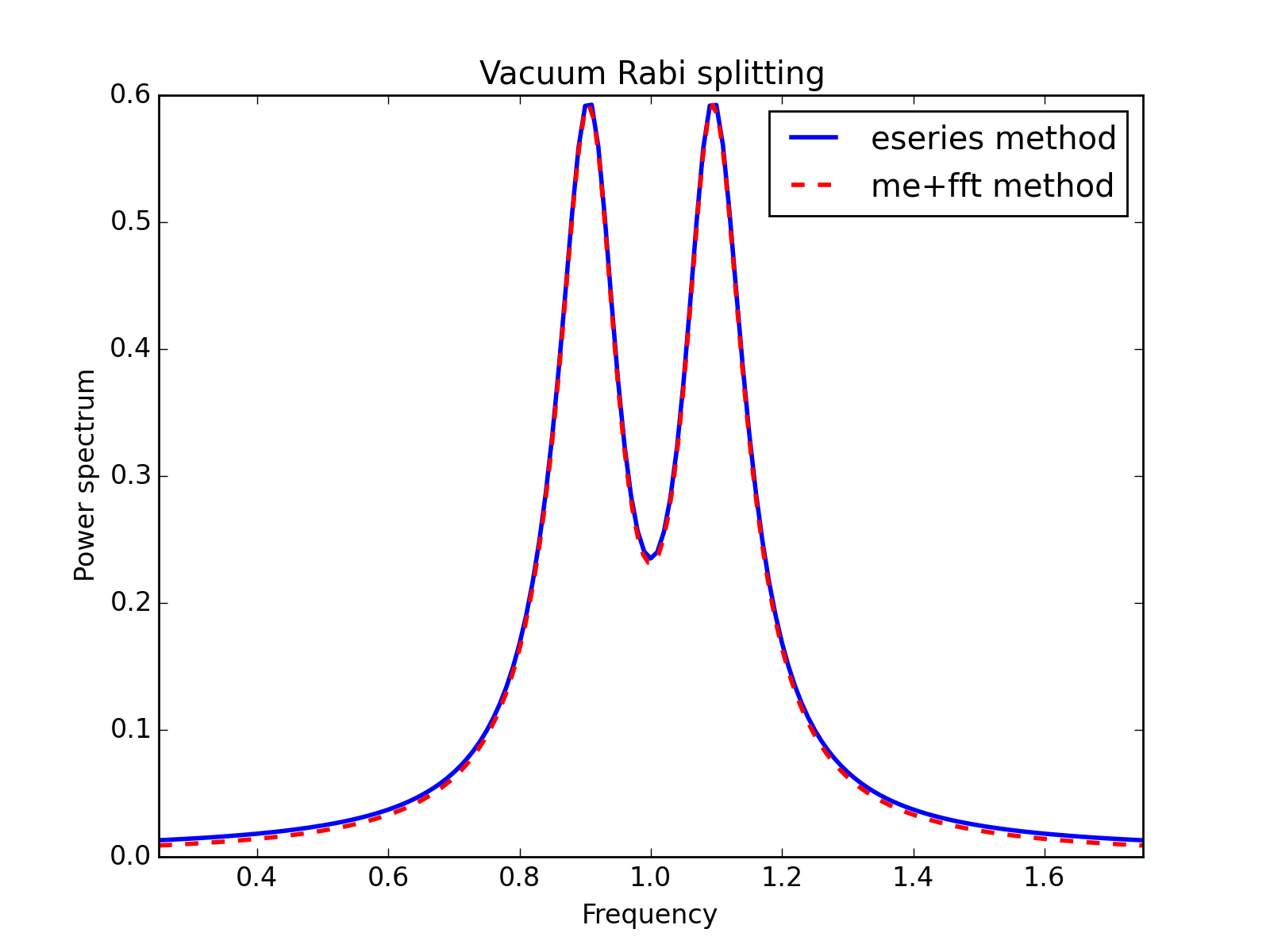
Emission spectrum
Given a correlation function \(\left<A(\tau)B(0)\right>\) we can define the corresponding power spectrum as
In QuTiP, we can calculate \(S(\omega)\) using either qutip.correlation.spectrum_ss, which first calculates the correlation function using the qutip.essolve.essolve solver and then performs the Fourier transform semi-analytically, or we can use the function qutip.correlation.spectrum_correlation_fft to numerically calculate the Fourier transform of a given correlation data using FFT.
The following example demonstrates how these two functions can be used to obtain the emission power spectrum.
import numpy as np
from qutip import *
import pylab as plt

N = 4                   # number of cavity fock states
wc = wa = 1.0 * 2 * np.pi  # cavity and atom frequency
g  = 0.1 * 2 * np.pi       # coupling strength
kappa = 0.75            # cavity dissipation rate
gamma = 0.25            # atom dissipation rate

# Jaynes-Cummings Hamiltonian
a  = tensor(destroy(N), qeye(2))
sm = tensor(qeye(N), destroy(2))
H = wc * a.dag() * a + wa * sm.dag() * sm + g * (a.dag() * sm + a * sm.dag())

# collapse operators
n_th = 0.25
c_ops = [np.sqrt(kappa * (1 + n_th)) * a, np.sqrt(kappa * n_th) * a.dag(), np.sqrt(gamma) * sm]

# calculate the correlation function using the mesolve solver, and then fft to
# obtain the spectrum. Here we need to make sure to evaluate the correlation
# function for a sufficient long time and sufficiently high sampling rate so
# that the discrete Fourier transform (FFT) captures all the features in the
# resulting spectrum.
tlist = np.linspace(0, 100, 5000)
corr = correlation_ss(H, tlist, c_ops, a.dag(), a)
wlist1, spec1 = spectrum_correlation_fft(tlist, corr)


# calculate the power spectrum using spectrum, which internally uses essolve
# to solve for the dynamics (by default)
wlist2 = np.linspace(0.25, 1.75, 200) * 2 * np.pi
spec2 = spectrum(H, wlist2, c_ops, a.dag(), a)

# plot the spectra
fig, ax = plt.subplots(1, 1)
ax.plot(wlist1 / (2 * np.pi), spec1, 'b', lw=2, label='eseries method')
ax.plot(wlist2 / (2 * np.pi), spec2, 'r--', lw=2, label='me+fft method')
ax.legend()
ax.set_xlabel('Frequency')
ax.set_ylabel('Power spectrum')
ax.set_title('Vacuum Rabi splitting')
ax.set_xlim(wlist2[0]/(2*np.pi), wlist2[-1]/(2*np.pi))
plt.show()
(Source code, png, hires.png, pdf)

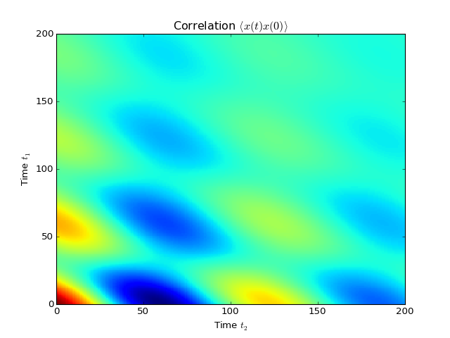
Non-steadystate correlation function
More generally, we can also calculate correlation functions of the kind \(\left<A(t_1+t_2)B(t_1)\right>\), i.e., the correlation function of a system that is not in its steadystate. In QuTiP, we can evoluate such correlation functions using the function qutip.correlation.correlation_2op_2t. The default behavior of this function is to return a matrix with the correlations as a function of the two time coordinates (\(t_1\) and \(t_2\)).
import numpy as np
from qutip import *
from pylab import *

times = np.linspace(0, 10.0, 200)
a = destroy(10)
x = a.dag() + a
H = a.dag() * a
alpha = 2.5
rho0 = coherent_dm(10, alpha)
corr = correlation_2op_2t(H, rho0, times, times, [np.sqrt(0.25) * a], x, x)

pcolor(corr)
xlabel(r'Time $t_2$')
ylabel(r'Time $t_1$')
title(r'Correlation $\left<x(t)x(0)\right>$')
show()
(Source code, png, hires.png, pdf)

However, in some cases we might be interested in the correlation functions on the form \(\left<A(t_1+t_2)B(t_1)\right>\), but only as a function of time coordinate \(t_2\). In this case we can also use the qutip.correlation.correlation_2op_2t function, if we pass the density matrix at time \(t_1\) as second argument, and None as third argument. The qutip.correlation.correlation_2op_2t function then returns a vector with the correlation values corresponding to the times in taulist (the fourth argument).
Example: first-order optical coherence function
This example demonstrates how to calculate a correlation function on the form \(\left<A(\tau)B(0)\right>\) for a non-steady initial state. Consider an oscillator that is interacting with a thermal environment. If the oscillator initially is in a coherent state, it will gradually decay to a thermal (incoherent) state. The amount of coherence can be quantified using the first-order optical coherence function \(g^{(1)}(\tau) = \frac{\left<a^\dagger(\tau)a(0)\right>}{\sqrt{\left<a^\dagger(\tau)a(\tau)\right>\left<a^\dagger(0)a(0)\right>}}\). For a coherent state \(|g^{(1)}(\tau)| = 1\), and for a completely incoherent (thermal) state \(g^{(1)}(\tau) = 0\). The following code calculates and plots \(g^{(1)}(\tau)\) as a function of \(\tau\).
import numpy as np
from qutip import *
from pylab import *

N = 15
taus = np.linspace(0,10.0,200)
a = destroy(N)
H = 2 * np.pi * a.dag() * a

# collapse operator
G1 = 0.75
n_th = 2.00  # bath temperature in terms of excitation number
c_ops = [np.sqrt(G1 * (1 + n_th)) * a, np.sqrt(G1 * n_th) * a.dag()]

# start with a coherent state
rho0 = coherent_dm(N, 2.0)

# first calculate the occupation number as a function of time
n = mesolve(H, rho0, taus, c_ops, [a.dag() * a]).expect[0]

# calculate the correlation function G1 and normalize with n to obtain g1
G1 = correlation_2op_2t(H, rho0, None, taus, c_ops, a.dag(), a)
g1 = G1 / np.sqrt(n[0] * n)

plot(taus, g1, 'b')
plot(taus, n, 'r')
title('Decay of a coherent state to an incoherent (thermal) state')
xlabel(r'$\tau$')
legend((r'First-order coherence function $g^{(1)}(\tau)$',
        r'occupation number $n(\tau)$'))
show()
(Source code, png, hires.png, pdf)
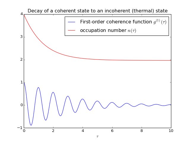
For convenience, the steps for calculating the first-order coherence function have been collected in the function qutip.correlation.coherence_function_g1.
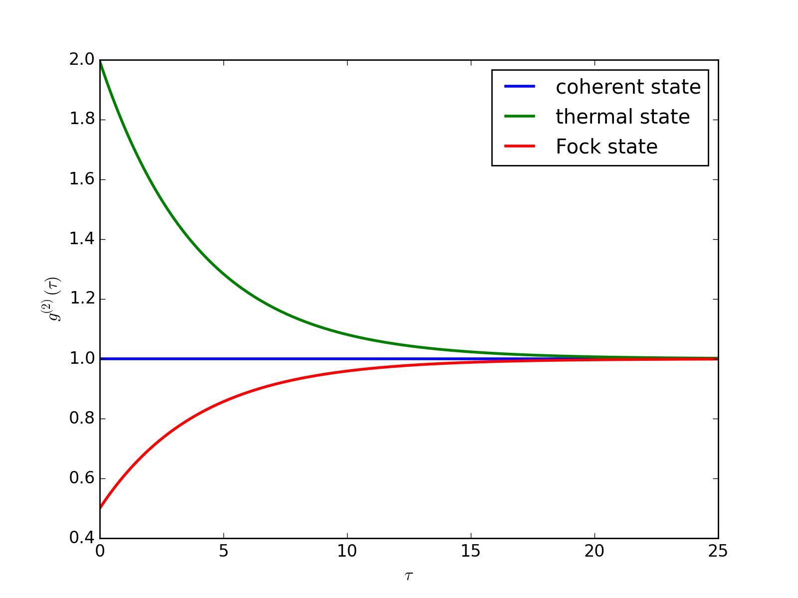
Example: second-order optical coherence function
The second-order optical coherence function, with time-delay \(\tau\), is defined as
For a coherent state \(g^{(2)}(\tau) = 1\), for a thermal state \(g^{(2)}(\tau=0) = 2\) and it decreases as a function of time (bunched photons, they tend to appear together), and for a Fock state with \(n\) photons \(g^{(2)}(\tau = 0) = n(n - 1)/n^2 < 1\) and it increases with time (anti-bunched photons, more likely to arrive separated in time).
To calculate this type of correlation function with QuTiP, we can use qutip.correlation.correlation_4op_1t, which computes a correlation function on the form \(\left<A(0)B(\tau)C(\tau)D(0)\right>\) (four operators, one delay-time vector).
The following code calculates and plots \(g^{(2)}(\tau)\) as a function of \(\tau\) for a coherent, thermal and fock state.
import numpy as np
from qutip import *
import pylab as plt

N = 25
taus = np.linspace(0, 25.0, 200)
a = destroy(N)
H = 2 * np.pi * a.dag() * a

kappa = 0.25
n_th = 2.0  # bath temperature in terms of excitation number
c_ops = [np.sqrt(kappa * (1 + n_th)) * a, np.sqrt(kappa * n_th) * a.dag()]

states = [{'state': coherent_dm(N, np.sqrt(2)), 'label': "coherent state"},
          {'state': thermal_dm(N, 2), 'label': "thermal state"},
          {'state': fock_dm(N, 2), 'label': "Fock state"}]

fig, ax = plt.subplots(1, 1)

for state in states:
    rho0 = state['state']

    # first calculate the occupation number as a function of time
    n = mesolve(H, rho0, taus, c_ops, [a.dag() * a]).expect[0]

    # calculate the correlation function G2 and normalize with n(0)n(t) to
    # obtain g2
    G2 = correlation_4op_1t(H, rho0, taus, c_ops, a.dag(), a.dag(), a, a)
    g2 = G2 / (n[0] * n)

    ax.plot(taus, np.real(g2), label=state['label'], lw=2)

ax.legend(loc=0)
ax.set_xlabel(r'$\tau$')
ax.set_ylabel(r'$g^{(2)}(\tau)$')
plt.show()
(Source code, png, hires.png, pdf)
For convenience, the steps for calculating the second-order coherence function have been collected in the function qutip.correlation.coherence_function_g2.