Dynamics Simulation Results
Important
In QuTiP 2, the results from all of the dynamics solvers are returned as Odedata objects. This unified and significantly simplified postprocessing of simulation results from different solvers, compared to QuTiP 1. However, this change also results in the loss of backward compatibility with QuTiP version 1.x. In QuTiP 3, the Result class has been renamed to Result, but for backwards compatibility an alias between Result and Odedata is provided.
The solver.Result Class
Before embarking on simulating the dynamics of quantum systems, we will first look at the data structure used for returning the simulation results to the user. This object is a qutip.solver.Result class that stores all the crucial data needed for analyzing and plotting the results of a simulation. Like the qutip.Qobj class, the Result class has a collection of properties for storing information. However, in contrast to the Qobj class, this structure contains no methods, and is therefore nothing but a container object. A generic Result object result contains the following properties for storing simulation data:
| Property | Description |
|---|---|
| result.solver | String indicating which solver was used to generate the data. |
| result.times | List/array of times at which simulation data is calculated. |
| result.expect | List/array of expectation values, if requested. |
| result.states | List/array of state vectors/density matrices calculated at times, if requested. |
| result.num_expect | The number of expectation value operators in the simulation. |
| result.num_collapse | The number of collapse operators in the simulation. |
| result.ntraj | Number of Monte Carlo trajectories run. |
| result.col_times | Times at which state collapse occurred. Only for Monte Carlo solver. |
| result.col_which | Which collapse operator was responsible for each collapse in in col_times. Only used by Monte Carlo solver. |
Accessing Result Data
To understand how to access the data in a Result object we will use an example as a guide, although we do not worry about the simulation details at this stage. Like all solvers, the Monte Carlo solver used in this example returns an Result object, here called simply result. To see what is contained inside result we can use the print function:
>>> print(result)
    Result object with mcsolve data.
    ---------------------------------
    expect = True
    num_expect = 2, num_collapse = 2, ntraj = 500
The first line tells us that this data object was generated from the Monte Carlo solver mcsolve (discussed in Monte Carlo Solver). The next line (not the --- line of course) indicates that this object contains expectation value data. Finally, the last line gives the number of expectation value and collapse operators used in the simulation, along with the number of Monte Carlo trajectories run. Note that the number of trajectories ntraj is only displayed when using the Monte Carlo solver.
Now we have all the information needed to analyze the simulation results. To access the data for the two expectation values one can do:
>>> expt0 = result.expect[0]
>>> expt1 = result.expect[1]
Recall that Python uses C-style indexing that begins with zero (i.e., [0] => 1st collapse operator data). Together with the array of times at which these expectation values are calculated:
>>> times = result.times
we can plot the resulting expectation values:
>>> plot(times, expt0, times, expt1)
>>> show()
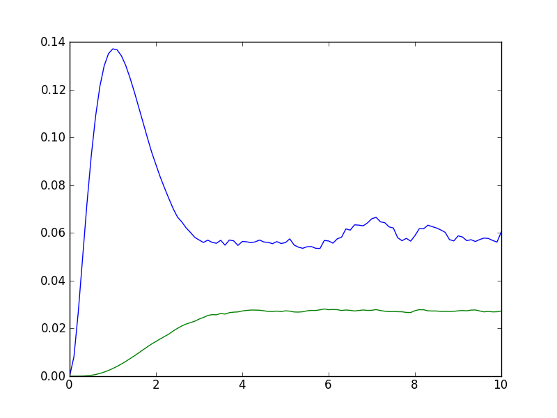
Data for expectation values extracted from the result Result object.
State vectors, or density matrices, as well as col_times and col_which, are accessed in a similar manner, although typically one does not need an index (i.e [0]) since there is only one list for each of these components. The one exception to this rule is if you choose to output state vectors from the Monte Carlo solver, in which case there are ntraj number of state vector arrays.
Saving and Loading Result Objects
The main advantage in using the Result class as a data storage object comes from the simplicity in which simulation data can be stored and later retrieved. The qutip.fileio.qsave and qutip.fileio.qload functions are designed for this task. To begin, let us save the data object from the previous section into a file called “cavity+qubit-data” in the current working directory by calling:
>>> qsave(result, 'cavity+qubit-data')
All of the data results are then stored in a single file of the same name with a ”.qu” extension. Therefore, everything needed to later this data is stored in a single file. Loading the file is just as easy as saving:
>>> stored_result = qload('cavity+qubit-data')
    Loaded Result object:
    Result object with mcsolve data.
    ---------------------------------
    expect = True
    num_expect = 2, num_collapse = 2, ntraj = 500
where stored_result is the new name of the Result object. We can then extract the data and plot in the same manner as before:
expt0 = stored_result.expect[0]
expt1 = stored_result.expect[1]
times = stored_result.times
plot(times, expt0, times, expt1)
show()

Data for expectation values from the stored_result object loaded from the result object stored with qutip.fileio.qsave
Also see Saving QuTiP Objects and Data Sets for more information on saving quantum objects, as well as arrays for use in other programs.