Stochastic Solver¶

Homodyne detection¶

Homodyne detection is an extension of the photocurrent method where the output is mixed with a strong external source allowing to get information about the phase of the system. With this method, the resulting detection rate depends is

\[ \begin{align}\begin{aligned}:label: jump_rate\\\tau = tr \left((\gamma^2 + \gamma (C+C^\dag) + C^\dag C)\rho \right)\end{aligned}\end{align} \]

With \(\gamma\), the strength of the external beam and \(C\) the collapse operator. When the beam is very strong \((\gamma >> C^\dag C)\), the rate becomes a constant term plus a term proportional to the quadrature of the system.

Closed system¶

In closed systems, the resulting stochastic differential equation is

(1)¶\[\delta \psi(t) = - i H \psi(t) \delta t - \sum_n \left( \frac{C_n^{+} C_n}{2} -\frac{e_n}{2} C_n + \frac{e_n^2}{8} \right) \psi \delta t + \sum_n \left( C_n - \frac{e_n}{2} \right) \psi \delta \omega\]

with

\[ \begin{align}\begin{aligned}:label: jump_rate\\e_n = \left<\psi(t)|C_n + C_n^{+}|\psi(t)\right>\end{aligned}\end{align} \]

Here \(\delta \omega\) is a Wiener increment.

In QuTiP, this is available with the function ssesolve.

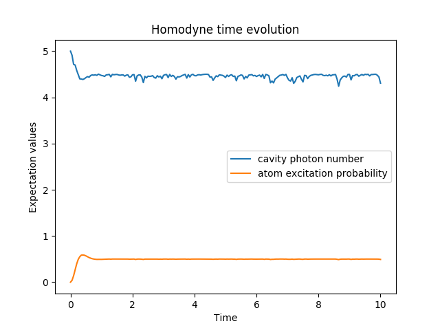
In [1]: times = np.linspace(0.0, 10.0, 201)

In [2]: psi0 = tensor(fock(2, 0), fock(10, 5))

In [3]: a  = tensor(qeye(2), destroy(10))

In [4]: sm = tensor(destroy(2), qeye(10))

In [5]: H = 2 * np.pi * a.dag() * a + 2 * np.pi * sm.dag() * sm + 2 * np.pi * 0.25 * (sm * a.dag() + sm.dag() * a)

In [6]: data = ssesolve(H, psi0, times, sc_ops=[np.sqrt(0.1) * a], e_ops=[a.dag() * a, sm.dag() * sm], method="homodyne")
Total run time:   0.03s

In [7]: figure()
Out[7]: <Figure size 640x480 with 0 Axes>

In [8]: plot(times, data.expect[0], times, data.expect[1])
Out[8]: 
[<matplotlib.lines.Line2D at 0x2b22694b2cf8>,
 <matplotlib.lines.Line2D at 0x2b22694b26a0>]

In [9]: title('Homodyne time evolution')
Out[9]: Text(0.5,1,'Homodyne time evolution')

In [10]: xlabel('Time')
Out[10]: Text(0.5,0,'Time')

In [11]: ylabel('Expectation values')
Out[11]: Text(0,0.5,'Expectation values')

In [12]: legend(("cavity photon number", "atom excitation probability"))
Out[12]: <matplotlib.legend.Legend at 0x2b226a6bd390>

In [13]: show()

Open system¶

In open systems, 2 types of collapse operators are considered, \(S_i\) represent the dissipation in the environment, \(C_i\) are monitored operators. The deterministic part of the evolution is the liouvillian with both types of collapses

(2)¶\[L(\rho(t)) = - i[H(t),\rho(t)] + \sum_n D(S_n, \rho) + \sum_i D(C_i, \rho),\]

with

(3)¶\[D(C, \rho) = \frac{1}{2} \left[2 C \rho(t) C^{+} - \rho(t) C^{+} C - C^{+} C \rho(t) \right].\]

The stochastic part is given by

(4)¶\[d_2 = \left(C \rho(t) + \rho(t) C^{+} - \rm{tr}\left(C \times \rho + \rho \times C^{+} \right)\rho(t) \right),\]

resulting in the stochastic differential equation

(5)¶\[\delta \rho(t) = L(\rho(t)) \delta t + d_2 \delta \omega\]

The function smesolve covert these cases in QuTiP.

Heterodyne detection¶

With heterodyne detection, two measurements are made in order to obtain information about 2 orthogonal quadratures at once.