Solving Problems with Time-dependent Hamiltonians
Methods for Writing Time-Dependent Operators
In the previous examples of quantum evolution, we assumed that the systems under consideration were described by time-independent Hamiltonians. However, many systems have explicit time dependence in either the Hamiltonian, or the collapse operators describing coupling to the environment, and sometimes both components might depend on time. The two main evolution solvers in QuTiP, qutip.mesolve and qutip.mcsolve, discussed in Lindblad Master Equation Solver and Monte Carlo Solver respectively, are capable of handling time-dependent Hamiltonians and collapse terms. There are, in general, three different ways to implement time-dependent problems in QuTiP:
- Function based: Hamiltonian / collapse operators expressed using [qobj, func] pairs, where the time-dependent coefficients of the Hamiltonian (or collapse operators) are expressed in the Python functions.
- String (Cython) based: The Hamiltonian and/or collapse operators are expressed as a list of [qobj, string] pairs, where the time-dependent coefficients are represented as strings. The resulting Hamiltonian is then compiled into C code using Cython and executed.
- Hamiltonian function (outdated): The Hamiltonian is itself a Python function with time-dependence. Collapse operators must be time independent using this input format.
Give the multiple choices of input style, the first question that arrises is which option to choose? In short, the function based method (option #1) is the most general, allowing for essentially arbitrary coefficients expressed via user defined functions. However, by automatically compiling your system into C code, the second option (string based) tends to be more efficient and will run faster. Of course, for small system sizes and evolution times, the difference will be minor. Although this method does not support all time-dependent coefficients that one can think of, it does support essentially all problems that one would typically encounter. If you can write you time-dependent coefficients using any of the following functions, or combinations thereof (including constants) then you may use this method:
'acos', 'acosh', 'asin', 'asinh', 'atan', 'atan2', 'atanh', 'ceil',
'copysign', 'cos', 'cosh', 'degrees', 'erf', 'erfc', 'exp', 'expm1',
'fabs', 'factorial', 'floor', 'fmod', 'frexp', 'fsum', 'gamma',
'hypot', 'isinf', 'isnan', 'ldexp', 'lgamma', 'log', 'log10', 'log1p',
'modf', 'pow', 'radians', 'sin', 'sinh', 'sqrt', 'tan', 'tanh', 'trunc'
Finally option #3, expressing the Hamiltonian as a Python function, is the original method for time dependence in QuTiP 1.x. However, this method is somewhat less efficient then the previously mentioned methods, and does not allow for time-dependent collapse operators. However, in contrast to options #1 and #2, this method can be used in implementing time-dependent Hamiltonians that cannot be expressed as a function of constant operators with time-dependent coefficients.
A collection of examples demonstrating the simulation of time-dependent problems can be found on the tutorials web page.
Function Based Time Dependence
A very general way to write a time-dependent Hamiltonian or collapse operator is by using Python functions as the time-dependent coefficients. To accomplish this, we need to write a Python function that returns the time-dependent coefficient. Additionally, we need to tell QuTiP that a given Hamiltonian or collapse operator should be associated with a given Python function. To do this, one needs to specify operator-function pairs in list format: [Op, py_coeff], where Op is a given Hamiltonian or collapse operator and py_coeff is the name of the Python function representing the coefficient. With this format, the form of the Hamiltonian for both mesolve and mcsolve is:
>>> H = [H0, [H1, py_coeff1], [H2, py_coeff2], ...]
where H0 is a time-independent Hamiltonian, while H1,``H2``, are time dependent. The same format can be used for collapse operators:
>>> c_ops = [[C0, py_coeff0], C1, [C2, py_coeff2], ...]
Here we have demonstrated that the ordering of time-dependent and time-independent terms does not matter. In addition, any or all of the collapse operators may be time dependent.
Note
While, in general, you can arrange time-dependent and time-independent terms in any order you like, it is best to place all time-independent terms first.
As an example, we will look at an example that has a time-dependent Hamiltonian of the form \(H=H_{0}-f(t)H_{1}\) where \(f(t)\) is the time-dependent driving strength given as \(f(t)=A\exp\left[-\left( t/\sigma \right)^{2}\right]\). The follow code sets up the problem:
from qutip import *
from scipy import *
# Define atomic states. Use ordering from paper
ustate = basis(3, 0)
excited = basis(3, 1)
ground = basis(3, 2)

# Set where to truncate Fock state for cavity
N = 2

# Create the atomic operators needed for the Hamiltonian
sigma_ge = tensor(qeye(N), ground * excited.dag())  # |g><e|
sigma_ue = tensor(qeye(N), ustate * excited.dag())  # |u><e|

# Create the photon operator
a = tensor(destroy(N), qeye(3))
ada = tensor(num(N), qeye(3))

# Define collapse operators
c_ops = []
# Cavity decay rate
kappa = 1.5
c_ops.append(sqrt(kappa) * a)

# Atomic decay rate
gamma = 6  # decay rate
# Use Rb branching ratio of 5/9 e->u, 4/9 e->g
c_ops.append(sqrt(5*gamma/9) * sigma_ue)
c_ops.append(sqrt(4*gamma/9) * sigma_ge)

# Define time vector
t = linspace(-15, 15, 100)

# Define initial state
psi0 = tensor(basis(N, 0), ustate)

# Define states onto which to project
state_GG = tensor(basis(N, 1), ground)
sigma_GG = state_GG * state_GG.dag()
state_UU = tensor(basis(N, 0), ustate)
sigma_UU = state_UU * state_UU.dag()

# Set up the time varying Hamiltonian
g = 5  # coupling strength
H0 = -g * (sigma_ge.dag() * a + a.dag() * sigma_ge)  # time-independent term
H1 = (sigma_ue.dag() + sigma_ue)  # time-dependent term
Given that we have a single time-dependent Hamiltonian term, and constant collapse terms, we need to specify a single Python function for the coefficient \(f(t)\). In this case, one can simply do:
def H1_coeff(t, args):
return 9 * exp(-(t / 5.) ** 2)
In this case, the return value dependents only on time. However, when specifying Python functions for coefficients, the function must have (t,args) as the input variables, in that order. Having specified our coefficient function, we can now specify the Hamiltonian in list format and call the solver (in this case qutip.mesolve):
H = [H0,[H1,H1_coeff]]
output = mesolve(H, psi0, t, c_ops, [ada, sigma_UU, sigma_GG])
We can call the Monte Carlo solver in the exact same way (if using the default ntraj=500):
>>> output = mcsolve(H, psi0, t, c_ops, [ada, sigma_UU, sigma_GG])
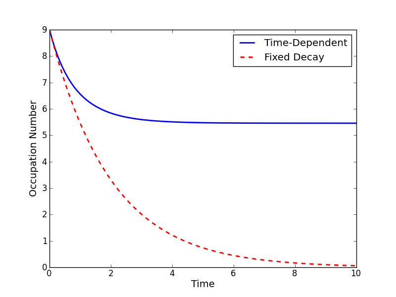
The output from the master equation solver is identical to that shown in the examples, the Monte Carlo however will be noticeably off, suggesting we should increase the number of trajectories for this example. In addition, we can also consider the decay of a simple Harmonic oscillator with time-varying decay rate:
from qutip import *
kappa = 0.5
def col_coeff(t, args):  # coefficient function
    return sqrt(kappa * exp(-t))
N = 10  # number of basis states
a = destroy(N)
H = a.dag() * a  # simple HO
psi0 = basis(N, 9)  # initial state
c_ops = [[a, col_coeff]]  # time-dependent collapse term
times = linspace(0, 10, 100)
output = mesolve(H, psi0, times, c_ops, [a.dag() * a])
A comparison of this time-dependent damping, with that of a constant decay term is presented below.
Using the args variable
In the previous example we hardcoded all of the variables, driving amplitude \(A\) and width \(\sigma\), with their numerical values. This is fine for problems that are specialized, or that we only want to run once. However, in many cases, we would like to change the parameters of the problem in only one location (usually at the top of the script), and not have to worry about manually changing the values on each run. QuTiP allows you to accomplish this using the keyword args as an input to the solvers. For instance, instead of explicitly writing 9 for the amplitude and 5 for the width of the gaussian driving term, we can make us of the args variable:
def H1_coeff(t, args):
    return args['A'] * exp(-(t/args['sigma'])**2)
or equivalently:
def H1_coeff(t, args):
    A = args['A']
    sig = args['sigma']
    return A * exp(-(t / sig) ** 2)
where args is a Python dictionary of key: value pairs args = {'A': a, 'sigma': b} where a and b are the two parameters for the amplitude and width, respectively. Of course, we can always hardcode the values in the dictionary as well args = {'A': 9, 'sigma': 5}, but there is much more flexibility by using variables in args. To let the solvers know that we have a set of args to pass we append the args to the end of the solver input:
>>> output = mesolve(H, psi0, times, c_ops, [a.dag() * a], args={'A': 9, 'sigma': 5})
or to keep things looking pretty:
args = {'A': 9, 'sigma': 5}
output = mesolve(H, psi0, times, c_ops, [a.dag() * a], args=args)
Once again, the Monte Carlo solver qutip.mcsolve works in an identical manner.
String Format Method
Note
You must have Cython installed on your computer to use this format. See Installation for instructions on installing Cython.
The string-based time-dependent format works in a similar manner as the previously discussed Python function method. That being said, the underlying code does something completely different. When using this format, the strings used to represent the time-dependent coefficients, as well as Hamiltonian and collapse operators, are rewritten as Cython code using a code generator class and then compiled into C code. The details of this meta-programming will be published in due course. however, in short, this can lead to a substantial reduction in time for complex time-dependent problems, or when simulating over long intervals. We remind the reader that the types of functions that can be used with this method is limited to:
['acos', 'acosh', 'asin', 'asinh', 'atan', 'atan2', 'atanh', 'ceil'
, 'copysign', 'cos', 'cosh', 'degrees', 'erf', 'erfc', 'exp', 'expm1'
, 'fabs', 'factorial', 'floor', 'fmod', 'frexp', 'fsum', 'gamma'
, 'hypot', 'isinf', 'isnan', 'ldexp', 'lgamma', 'log', 'log10', 'log1p'
, 'modf', 'pow', 'radians', 'sin', 'sinh', 'sqrt', 'tan', 'tanh', 'trunc']
Like the previous method, the string-based format uses a list pair format [Op, str] where str is now a string representing the time-dependent coefficient. For our first example, this string would be '9 * exp(-(t / 5.) ** 2)'. The Hamiltonian in this format would take the form:
>>> H = [H0, [H1, '9 * exp(-(t / 5.) ** 2)']]
Notice that this is a valid Hamiltonian for the string-based format as exp is included in the above list of suitable functions. Calling the solvers is the same as before:
>>> output = mesolve(H, psi0, times, c_ops, [a.dag() * a])
We can also use the args variable in the same manner as before, however we must rewrite our string term to read: 'A * exp(-(t / sig) ** 2)':
H = [H0, [H1, 'A * exp(-(t / sig) ** 2)']]
args = {'A': 9, 'sig': 5}
output = mesolve(H, psi0, times, c_ops, [a.dag()*a], args=args)
Important
Naming your args variables e or pi will mess things up when using the string-based format.
Collapse operators are handled in the exact same way.
Function Based Hamiltonian
In the previous version of QuTiP, the simulation of time-dependent problems required writing the Hamiltonian itself as a Python function. However, this method does not allow for time-dependent collapse operators, and is therefore more restrictive. Furthermore, it is less efficient than the other methods for all but the most basic of Hamiltonians (see the next section for a comparison of times.). In this format, the entire Hamiltonian is written as a Python function:
def Hfunc(t, args):
    H0 = args[0]
    H1 = args[1]
    w = 9 * exp(-(t/5.)**2)
    return H0 - w * H1
where the args variable must always be given, and is now a list of Hamiltonian terms: args=[H0, H1]. In this format, our call to the master equation is now:
>>> output = mesolve(Hfunc, psi0, times, c_ops, [a.dag() * a], args=[H0, H1])
We cannot evaluate time-dependent collapse operators in this format, so we can not simulate the previous harmonic oscillator decay example.
A Quick Comparison of Simulation Times
Here we give a table of simulation times for the single-photon example using the different time-dependent formats and both the master equation and Monte Carlo solver.
| Format | Master Equation | Monte Carlo |
|---|---|---|
| Python Function | 2.1 sec | 27 sec |
| Cython String | 1.4 sec | 9 sec |
| Hamiltonian Function | 1.0 sec | 238 sec |
For the current example, the table indicates that the Hamiltonian function method is in fact the fastest when using the master equation solver. This is because the simulation is quite small. In contrast, the Hamiltonian function is over 26x slower than the compiled string version when using the Monte Carlo solver. In this case, the 500 trajectories needed in the simulation highlights the inefficient nature of the Python function calls.
Reusing Time-Dependent Hamiltonian Data
Note
This section covers a specialized topic and may be skipped if you are new to QuTiP.
When repeatedly simulating a system where only the time-dependent variables, or initial state change, it is possible to reuse the Hamiltonian data stored in QuTiP and there by avoid spending time needlessly preparing the Hamiltonian and collapse terms for simulation. To turn on the the reuse features, we must pass a qutip.Options object with the rhs_reuse flag turned on. Instructions on setting flags are found in Setting Options for the Dynamics Solvers. For example, we can do:
H = [H0, [H1, 'A * exp(-(t / sig) ** 2)']]
args = {'A': 9, 'sig': 5}
output = mcsolve(H, psi0, times, c_ops, [a.dag()*a], args=args)
opts = Options(rhs_reuse=True)
args = {'A': 10, 'sig': 3}
output = mcsolve(H, psi0, times, c_ops, [a.dag()*a], args=args, options=opts)
In this case, the second call to qutip.mcsolve takes 3 seconds less than the first. Of course our parameters are different, but this also shows how much time one can save by not reorganizing the data, and in the case of the string format, not recompiling the code. If you need to call the solvers many times for different parameters, this savings will obviously start to add up.
Running String-Based Time-Dependent Problems using Parfor
Note
This section covers a specialized topic and may be skipped if you are new to QuTiP.
In this section we discuss running string-based time-dependent problems using the qutip.parfor function. As the qutip.mcsolve function is already parallelized, running string-based time dependent problems inside of parfor loops should be restricted to the qutip.mesolve function only. When using the string-based format, the system Hamiltonian and collapse operators are converted into C code with a specific file name that is automatically genrated, or supplied by the user via the rhs_filename property of the qutip.Options class. Because the qutip.parfor function uses the built-in Python multiprocessing functionality, in calling the solver inside a parfor loop, each thread will try to generate compiled code with the same file name, leading to a crash. To get around this problem you can call the qutip.rhs_generate function to compile simulation into C code before calling parfor. You must then set the qutip.Odedata object rhs_reuse=True for all solver calls inside the parfor loop that indicates that a valid C code file already exists and a new one should not be generated. As an example, we will look at the Landau-Zener-Stuckelberg interferometry example that can be found in the notebook “Time-dependent master equation: Landau-Zener-Stuckelberg inteferometry” in the tutorials section of the QuTiP web site.
To set up the problem, we run the following code:
from qutip import *

# set up the parameters and start calculation
delta    = 0.1  * 2 * pi  # qubit sigma_x coefficient
w        = 2.0  * 2 * pi  # driving frequency
T        = 2 * pi / w     # driving period
gamma1   = 0.00001        # relaxation rate
gamma2   = 0.005          # dephasing  rate
eps_list = linspace(-10.0, 10.0, 501) * 2 * pi  # epsilon
A_list   = linspace(0.0, 20.0, 501) * 2 * pi    # Amplitude

# pre-calculate the necessary operators
sx = sigmax(); sz = sigmaz(); sm = destroy(2); sn = num(2)
# collapse operators
c_ops = [sqrt(gamma1) * sm, sqrt(gamma2) * sz]  # relaxation and dephasing

# setup time-dependent Hamiltonian (list-string format)
H0 = -delta / 2.0 * sx
H1 = [sz, '-eps / 2.0 + A / 2.0 * sin(w * t)']
H_td = [H0, H1]
Hargs = {'w': w, 'eps': eps_list[0], 'A': A_list[0]}
where the last code block sets up the problem using a string-based Hamiltonian, and Hargs is a dictionary of arguments to be passed into the Hamiltonian. In this example, we are going to use the qutip.propagator and qutip.propagator.propagator_steadystate to find expectation values for different values of \(\epsilon\) and \(A\) in the Hamiltonian \(H = -\frac{1}{2}\Delta\sigma_x -\frac{1}{2}\epsilon\sigma_z- \frac{1}{2}A\sin(\omega t)\).
We must now tell the qutip.mesolve function, that is called by qutip.propagator to reuse a pre-generated Hamiltonian constructed using the qutip.rhs_generate command:
# ODE settings (for reusing list-str format Hamiltonian)
opts = Options(rhs_reuse=True)
# pre-generate RHS so we can use parfor
rhs_generate(H_td, c_ops, Hargs, name='lz_func')
Here, we have given the generated file a custom name lz_func, however this is not necessary as a generic name will automatically be given. Now we define the function task that is called by parfor:
# a task function for the for-loop parallelization:
# the m-index is parallelized in loop over the elements of p_mat[m,n]
def task(args):
    m, eps = args
    p_mat_m = zeros(len(A_list))
    for n, A in enumerate(A_list):
        # change args sent to solver, w is really a constant though.
        Hargs = {'w': w, 'eps': eps,'A': A}
        U = propagator(H_td, T, c_ops, Hargs, opts) #<- IMPORTANT LINE
        rho_ss = propagator_steadystate(U)
        p_mat_m[n] = expect(sn, rho_ss)
    return [m, p_mat_m]
Notice the Options opts in the call to the qutip.propagator function. This is tells the qutip.mesolve function used in the propagator to call the pre-generated file lz_func. If this were missing then the routine would fail.